Troubleshooting Dask GroupBy
Dask DataFrames are amazing for interactively exploring large datasets. However, using them on big datasets can be a little tricky. You’ve probably already hit a KilledWorker exception trying to do a GroupBy. If you haven’t, you will soon!
The goal of this article is to arm you with a set of options to try if your GroupBy fails. First, we’ll take a deep dive into how DataFrame GroupBy Aggregations are implemented. This is necessary to understand how to work around any obstacles you stumble upon.
Dask GroupBy Aggregation
Dask GroupBy aggregations1 use the apply_concat_apply() method, which applies 3 functions, a chunk(), combine() and an aggregate() function to a dask.DataFrame. This is a very powerful paradigm because it enables you to build your own custom aggregations by supplying these functions. We will be referring to these functions in the example.
- chunk : This method is applied to each partition of the Dask DataFrame.
- combine: Outputs from the
chunk()step are concatenated, and then combined together withcombine(). - aggregate: Outputs from the
combine()step are concatenated, and then aggregated withaggregate(). This is the last step. After this transformation, your result is complete.
Dask GroupBy Aggregation: The Simplest Example
In this example, we’ll walk through a Dask GroupBy with default parameters to show how the algorithm works. We’re using a dummy dataset that has been split into 4 partitions. We’ve chosen numerical values for score to have separate decimal places to make it obvious when data is being aggregated.
This example applies the following transformation:
df.groupby('animal')[['score']].sum().compute()
The Dask GroupBy Aggregation breaks the algorithm into chunk(), combine() and aggregate() steps. In this case (the simplest one), we only use the chunk() and aggregate() steps. This particular aggregation is elegant in that each of these steps is implemented in the same way, by grouping by the animal and summing the score (df.groupby('animal')['zscore'].sum()). By summing the partitions and then summing those sums, we can compute the desired result. Other algorithms like var() require different operations at the different stages. This diagram lays out the relevant operations, and shows us what the data looks like every step of the way.
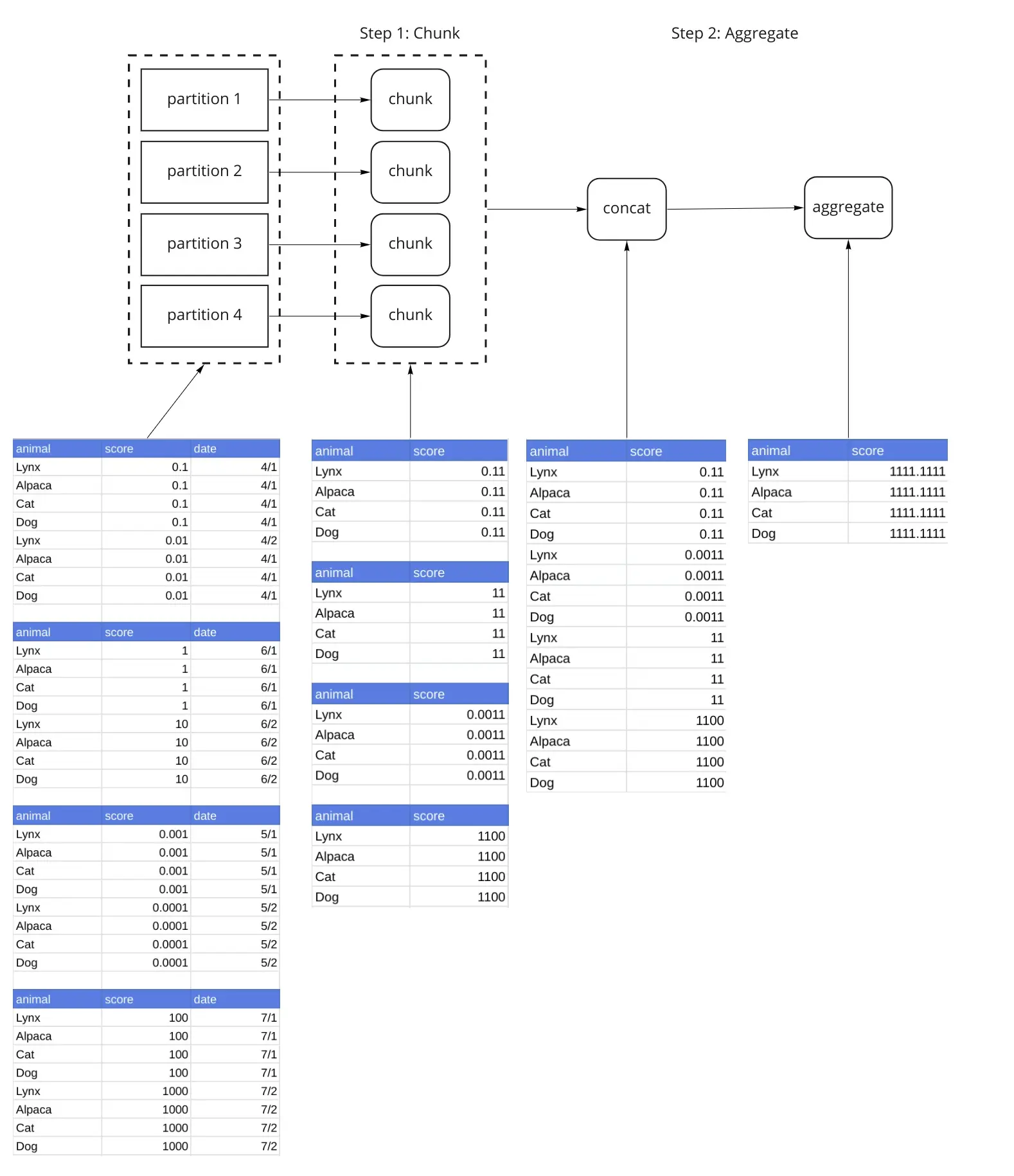
Our sample dataset has been split up into 4 partitions. Step 1 applies the chunk() function to each partition. This is an important step because its output is a reduction, and is much smaller than the original partition. Step 2 concatenates the outputs of Step 1 into a single dataframe, and then applies the aggregate() function to the result.
Issues
The simple case returns 1 partition with the entire result in it. If your GroupBy results in a small dataframe, this approach is great. If your GroupBy results in a large dataframe (if you have a large number of groups), you’ll run out of memory, which often manifests itself in KilledWorker exceptions.
Dealing with Memory: split_out
Dask provides 2 parameters, split_out and split_every to control the data flow. split_out controls the number of partitions that are generated. If we set split_out=4, the group by will result in 4 partitions, instead of 1. We’ll get to split_every later. Let’s redo the previous example with split_out=4.
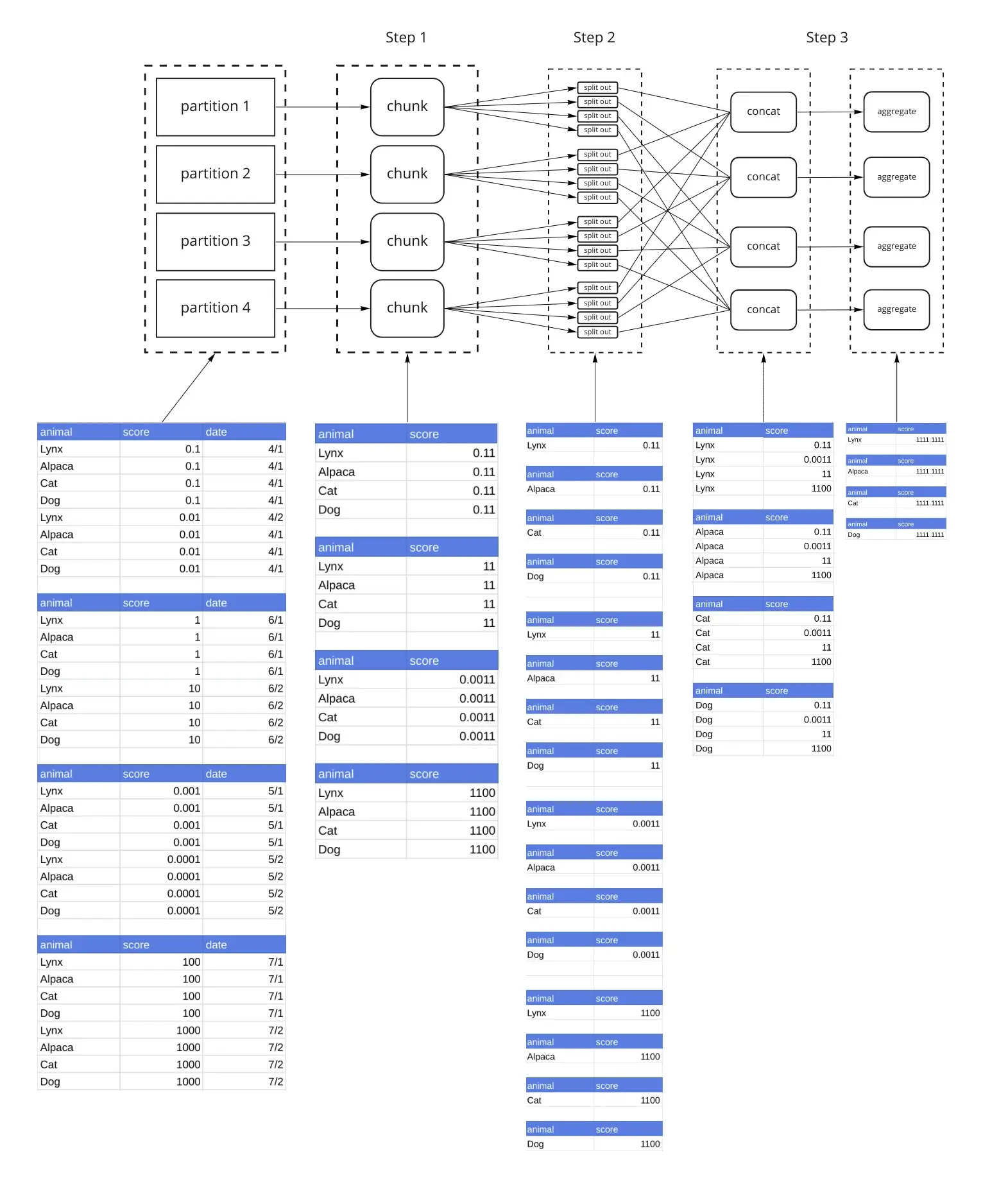
Step 1 is the same as the previous example. The output of Step 1 (applying the chunk() function) is 1 dataframe per partition. Step 2 breaks each of those dataframes into split_out=4 dataframes by hashing the groups. Looking at the diagram, you’ll see that the Nth dataframe from each partition has the same animal in it. That consistency is the objective of the hashing. We’ll refer to each group as a shard (Shard 1 contains the 1st DataFrame from each partition, Shard 2 contains the 2nd DataFrame from each partition, and so on). Step 3 concatenates all dataframes that make up each Shard (again using this hashing) such that the data from the same animals end up in the same dataframe. Then the aggregate() function is applied. The result is now a Dask DataFrame made up of split_out=4 partitions.
Advanced Options: split_every
In the previous example, Step 3, Dask concatenated data by shard, for every partition. By default, Dask will concatenate data by shard for up to 8 partitions at a time. Since our dataset only has 4 partitions, all the data was handled at once. Let’s re-run the previous example, with split_every=2. Everything up to Step 2 is the same.
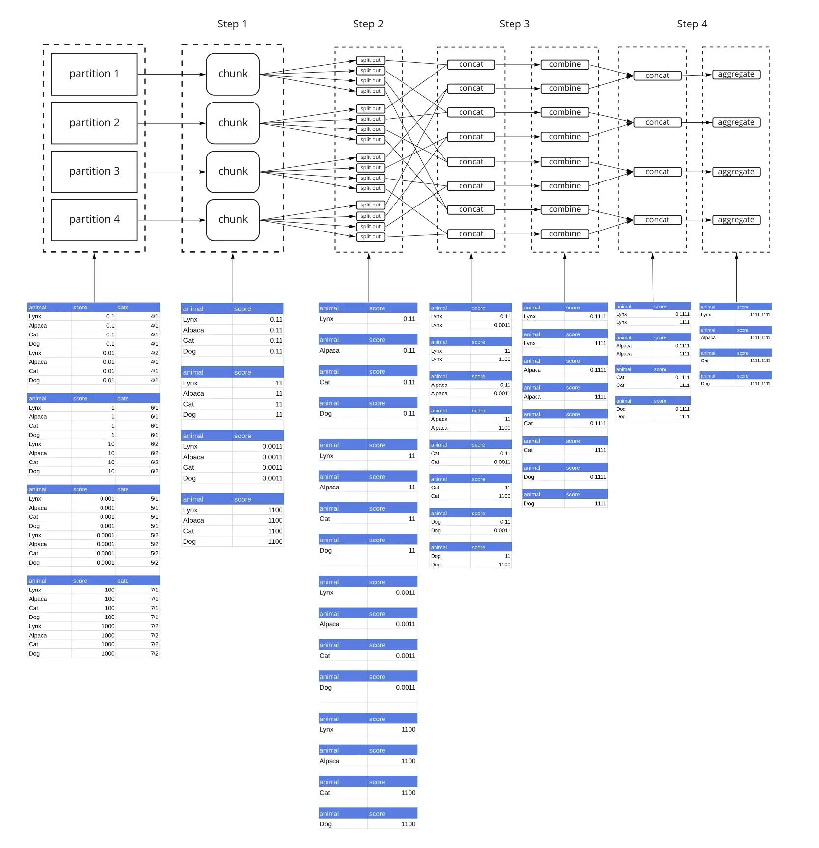
With split_every=2, instead of concatenating all dataframes from a single shard (in our example each shard has 4 dataframes), we concatenate them 2 at a time, and then combine them with the combine() function in Step 3. Step 4 concatenates those results and then calls aggregate(). The reduction with combine() and finally aggregate() is a tree reduction. Because we only have 4 partitions, we can complete this operation in 1 combine() step, and 1 aggregate() step. However if we had 8 partitions, there would be 2 combine() steps and 1 aggregate() step. aggregate() is always the last step.
What Do We Do About It
There are really only 2 things that can be done. I know this may seem a bit anti-climactic, given the length explanation we just went through about how the algorithm works, however understanding the algorithm is important for understanding how to tune it.
Tune split_out
The split_out parameter can be passed into the aggregation function.
ddf.groupby('animal')['scores'].sum(split_out=100)
This section is going to be a bit approximate and hand-wavy. Ultimately you’re going to need to experiment with your dataset and figure out what parameters work. This section may provide you with some guidance on how to think about it.
Understanding your data
How many groups am I going to have? Hopefully you understand your data well enough to get a rough estimate for the number of groups that will be in your result. If not, you may need to compute it somehow. So for example, I have a dataset with 50 million animals. I take a subset of the data, execute the computation, and observe that my result has 5 million animals and takes 500 mb in memory. 5 million animals is 1/10th of the 50 million I have in the dataset, so my final result will be roughly 5GB.
Partition Sizes
Partition sizing is a different topic that won’t be covered here. In general you should size your partitions so that many partitions can fit on a worker but ideal partition sizes depend on how much memory your workers have.
Let’s say I have 8GB workers. If my final result is 5GB, I could set split_out to be 5, so that each 1GB result fits comfortably on the worker. However, the default split_every parameter is set to 8. If every partition is 1GB, in the worst case I could be concatenating 8GB - which would blow out my 8GB worker. Instead, I select split_out to be 25 so that each partition is 200MB.
Reality won’t be this precise. Exact memory usage is going to depend on how your data is laid out between different machines, and how much memory is used in the actual pandas computation itself. If your data is sorted according to your groupby column, your memory usage will be close to ideal. If you have data from every group on every machine, your memory usage will be closer to the worst case scenario. But this approach can serve as a rough guidelines to choosing split_out .
I don’t recommend tuning split_every. It’s much easier to tune a single parameter, and the default value of 8 is similar to how much extra memory head room you would want in your Dask workers.
Use map_partitions Instead
map_partitions() is a method on a Dask DataFrame (it is also used in other Dask collections) that applies a function to all partitions of the Dask DataFrame, and then builds another Dask DataFrame over those results.
Using map_partitions() is only a good strategy if your data is already sorted by one of the fields you wish to group by. In this example dataset, if my data is already sorted by animal, and I know that all cats are in one partition, and all dogs are in another partition, then I know that I don’t need data from other partitions in order to compute statistics about each animal. This means I can replace
ddf.groupby('animal')['scores'].sum()
with
ddf.map_partitions(lambda x: x.groupby('animal')['scores'].sum()
Don’t sort your data
If my data is not sorted, I could sort it using set_index() . Then I can apply map_partitions() . This probably isn’t worth it. The data movement in a groupby aggregation should be less than the data movement in set_index() because the chunk() operation, which is the first step, reduces the data volume significantly.
Don’t use GroupBy and then Apply
map_partition is how a Dask GroupBy with an Apply is implemented when the data is already sorted. This means I could write my aggregation as
ddf.groupby('animal').apply(lambda x: x.sum())
This will likely be much slower than the original example, purely because pandas groupby applys are much slower than groupby aggregations.
Conclusion
Dask does a lot in order to implement GroupBy aggregations on a cluster. In most cases, it works really well out of the box. When it doesn’t, you can tune split_out to make Dask produce smaller chunks. If your data is already sorted, you can implement the operation more efficiently with map_partitions(). The actual algorithm can be a bit tricky to understand, but understanding it can help you gain intuition about how to tune the parameters.
the Dask custom Aggregation object uses slightly different terminology:
chunk(),aggregate()andfinalize(). If you end up implementing your own aggregations, you’ll want to use this object. However for this article, we’re sticking to the terminology forapply_concat_apply()because it’s closer to the memory issues that we’re trying to solve. ↩︎