
This article was published when data science tooling like Dask and R was a primary focus for Saturn Cloud. Today, Saturn Cloud is the enterprise AI platform for any GPU infrastructure.
Introducing a new Python package: dask-pytorch-ddp
This tutorial is run on the Saturn Cloud platform, which makes Dask clusters available at the click of a button to users. If you need access to clusters so you can try out the steps below, we have a free version
Data parallelism within a single machine is a reasonably well-documented method for optimizing deep learning training performance, particularly in PyTorch . However, taking the step from one machine to training a single neural net on many machines at once can seem difficult and complicated.
This tutorial will demonstrate first, that GPU cluster computing to
conduct transfer learning allows the data scientist to significantly
improve the effective learning of a model; and second, that implementing
this in Python is not as hard or scary as it sounds, especially with our
new library, dask-pytorch-ddp
We are going to use the same dataset that we used in our PyTorch parallelized inference tutorial, the Stanford Dogs dataset. Instead of using Resnet50 as it is out of the box, we’ll improve it with transfer learning. In normal cases, this task can be very time consuming and resource-intensive, but today you are going to find out how to make it learn better and faster with parallelization.
New to parallelized PyTorch?
In addition to the information provided here, we highly recommend users who are new to parallelized PyTorch visit some of the official documentation and excellent existing tutorials:
- Overview of Distributed PyTorch
- Writing Distributed Applications with PyTorch
- Distributed Data Parallel on PyTorch
- Getting Started with Distributed Data Parallel
- Distributed Data Parallel Docs
- Training Neural Nets on Larger Batches: Practical Tips for 1-GPU, Multi-GPU & Distributed setups by Thomas Wolf
Introducing Concepts
Before we dive into working on this, we should go over the underlying concepts around how parallelization is made possible in PyTorch.
torch.nn.parallel.DistributedDataParallel / DDP
DistributedDataParallel is PyTorch’s native structure for parallel model training on multiple machines. There’s a lot to know about how this works, and we can’t cover it all here, but we have a summary overview to get you started.
It may help to actually start by discussing DataParallel, which is the single-machine parallelization tool that PyTorch provides. This is really enabling the same parallel training, just on a single machine, and DistributedDataParallel then extends this to be able to work on multiple GPU machines.
The official PyTorch documentation tells us this:
This container parallelizes the application of the given module by splitting the input across the specified devices by chunking in the batch dimension (other objects will be copied once per device). In the forward pass, the module is replicated on each device, and each replica handles a portion of the input. During the backwards pass, gradients from each replica are summed into the original module.
Clear as mud, right? Let’s try to break it down.
This container parallelizes the application of the given module
This is just indicating that we’re parallelizing a deep learning workflow – transfer learning in our case.
by splitting the input across the specified devices by chunking in the batch dimension
Input for a transfer learning workflow is the dataset! Ok, so it is chunking our image batches and that’s what gets to be parallel.
(other objects will be copied once per device)
Eg, our starting model, if any (Resnet50 for us) doesn’t get broken up at all. Good to know.
In the forward pass, the module is replicated on each device, and each replica handles a portion of the input.
Ok, so the training task, our module, is replicated on each device. We have multiple copies of the job working simultaneously, and each one gets a chunk of the input images rather than the entire dataset.
During the backwards pass, gradients from each replica are summed into the original module.
And then each of these duplicate tasks passes the results (the gradients) back home to the original! The learning is happening out in the workers/child processes, and then they all return the results to the original module/training process to be aggregated.
The essential difference with DDP, then, is that it is optimized for multiple machines instead of a single machine with multiple threads. It’s able to communicate across different machines effectively, so we can use a GPU cluster for our computation.
Still with me? It’s reasonable to find this all a little confusing!
If you are still having any trouble understanding the process, it may help to think of all our workers as individuals working on the same puzzle problem. At the end of the epoch, they all hand their findings back to the master node, which combines the partial solutions each one has submitted. Then everyone gets a copy of this combined solution, which is still not complete, and they start working on it again for another epoch. The difference is that now they have a head start thanks to everyone’s combined work.
You could just have one person doing the work, for sure – and they might eventually even reach the same overall result. But they’re going to need a lot more time to get there, and the results will be worse at the outset. The group’s progress solving the problem will be better from the get-go, because every worker is going to have a slightly different strategy for solving, so you’re getting multiple approaches combined at the same time.
We’re not necessarily creating results that would be impossible with a single node, but we’re getting better results, faster, and will be able to stop training a lot sooner.
Taking PyTorch to the Cluster
If you’ve worked through any of our other tutorials that involve Dask
clusters on Saturn Cloud, you have read a little about the
commands used for instructing the client, aka our
Dask cluster. We’re using that very same functionality here under the
hood of dask-pytorch-ddp to take our distributed PyTorch job from the single worker to the
cluster.
torch.distributed.init_process_group
As the official PyTorch documentation tells
us, a Process Group is required for the workers to communicate with each
other and coordinate the work being completed. As a result, creating a
process group is a vital first step in the setup. We have handled this
for you in dask-pytorch-ddp,
where a function called dispatch.run is
provided, which we explain in the next section. You just supply a
function that contains the PyTorch training steps and the function takes
care of passing the work out to the cluster
appropriately.
dask-pytorch-ddp.dispatch.run
This particular function is pretty instrumental to the task we are undertaking, so we’ll look at
it just for a moment and explain how it works. (If you are very
interested in the details, the link above takes you to the full codebase
for dask-pytorch-ddp.)
Inside this function, the client is doing a few key things:
- Retrieving information about your particular Dask cluster, e.g. number of workers and sizes.
- Producing a list of the jobs you want to run, e.g. a training task for every worker in the cluster.
- Reserving this list in memory until you indicate that computations should begin.
- Creating and destroying the Process Group as needed, so that your tasks all communicate correctly.
As a result, if you ever run into challenges regarding your cluster and its interpretation/understanding of instructions, this function may be a helpful place to start.
See It In Action
Now that we have a general understanding of our tools, we can actually build our code to run this transfer learning task.
Data Setup
One thing that you might realize when contemplating this problem is
that loading image data from S3, as we do, might be slow – even the
slowest part of our task! We thought that too, which is why we wrote an
extension of the PyTorch Dataset class for this work. In
dask-pytorch-ddp you’ll find this class named S3ImageFolder. This
isn’t required for the workflow to operate, but it makes a huge
difference in the speed at which your workflow can
perform.
The arguments it requires are your S3 bucket name (string), your file prefix inside the bucket, and then any PyTorch transformations you wish to use. See below for an example of it in context. This way, any sort of file you have inside the S3 bucket can be loaded in highly parallel fashion, transformed efficiently, and then returned as a Dataset class object for use in other PyTorch tasks. We think you’ll be really impressed with the speed of processing this allows!
def prepro_batches(bucket, prefix):
    '''Create the S3ImageFolder Dataset object, apply transformations.'''
    transform = transforms.Compose([
    transforms.Resize(256),
    transforms.CenterCrop(250),
    transforms.ToTensor()])
    whole_dataset = data.S3ImageFolder(bucket, prefix, transform=transform)
    return whole_dataset
Split Samples
Of course, we want to do our due diligence when training this model, so we want to create train and evaluation splits of data to ensure that the improvements we’re seeing are valid and not overfitting.
Notice that the DataLoader objects here are being explicitly defined to use multiprocessing – this means we can take full advantage of parallelization to make our image ingestion faster when we finally call it in our training job function (described below).
def get_splits_parallel(train_pct, data, batch_size):
    '''Select two samples of data for training and evaluation'''
    classes = data.classes
    train_size = math.floor(len(data) * train_pct)
    indices = list(range(len(data)))
    np.random.shuffle(indices)
    train_idx = indices[:train_size]
    test_idx = indices[train_size:len(data)]

    train_sampler = SubsetRandomSampler(train_idx)
    test_sampler = SubsetRandomSampler(test_idx)

    train_loader = torch.utils.data.DataLoader(data, sampler=train_sampler, batch_size=batch_size, num_workers=num_workers, multiprocessing_context=mp.get_context('fork'))
    test_loader = torch.utils.data.DataLoader(data, sampler=train_sampler, batch_size=batch_size, num_workers=num_workers, multiprocessing_context=mp.get_context('fork'))

    return train_loader, test_loader
Setting Up Results Handling
We have one more new class to instantiate here, so that we can efficiently monitor the performance of our training task.
key = uuid.uuid4().hex
rh = results.DaskResultsHandler(key)
The DaskResultsHandler
class object has a few very useful methods, which we’ll take full
advantage of. The essential purpose of this class is to organize our
model’s training tasks and monitor the performance statistics for
us.
One of the methods is submit_result. This
method accepts a path (where we want results saved) and data (in our
case, some JSON that tells us the current performance of the model) and
handles all the work of organizing that for us.
rh.submit_result(
    f"worker/.json",
    json.dumps({'loss': loss.item(),
    'learning_rate':current_lr,
    'correct':correct,
    'epoch': epoch,
    'count': count,
    'worker': worker_rank,
    'sample': 'train'})
)
Another of the useful methods here is process_results,
which accepts a directory, a list of job futures, and some error
handling instructions. After we have created our futures (delayed jobs
assigned to workers on the cluster), we use this to formally kick off
all those tasks and make computations begin. In short, this task is the
last step once all our work is defined, organized, and ready to
run.
rh.process_results(
    "/home/data/parallel/ten_workers",
    futures,
    raise_errors=False)
Training Pipeline
This stage of the job, then, will be quite familiar to those who work in PyTorch on transfer learning or model training. We’re just going to write our model task, just as we might for single node work, and wrap it in a function so that it can be handed out to the workers.
We will look at this function in pieces first, then put it all together at the end before we run it.
Collect Model
To prepare the model, we need to grab it from torchvision first and
then we can pass it to the GPU compute resources. Then we’ll wrap it in DDP
as we talked about earlier.
...
device = torch.device(0)
net = models.resnet50(pretrained=True)
model = net.to(device)
device_ids = [0]
model = DDP(model, device_ids=device_ids)
...
Set Model Parameters
Excellent. Now we can establish the regular pieces that a PyTorch model task will require- our loss function, optimizer, and learning rate scheduler.
...
criterion = nn.CrossEntropyLoss().cuda()
lr = base_lr * dist.get_world_size()
optimizer = optim.SGD(model.parameters(), lr=lr, momentum=0.9)
scheduler = lr_scheduler.ReduceLROnPlateau(optimizer, mode = 'min', patience = 2)
...
You may notice I am choosing a learning rate scheduler that waits for
plateau of the loss function before shifting – this is a matter of
preference, and you could certainly use a step learning rate scheduler
(StepLR) here with no ill effects. It’s a matter of what works
best for your data and base model.
Retrieve Data from S3 and Process
Now, we collect our data. We need to initialize the data loader
objects, using our S3ImageFolder class
and the train/test splits, and name our data loaders for later
reference. The DataLoader class allows us to lazily load the images when
our training loop is ready for them – a major asset for this
work.
...
whole_dataset = prepro_batches(bucket, prefix)
train, val = get_splits_parallel(train_pct, whole_dataset, batch_size=batch_size)
dataloaders = {'train' : train, 'val': val}
...
Training Iterations
At this point, we’re ready to begin iteration over the number of epochs we have chosen. Here we set the model to training mode, and loop over the batches of images that our “train” DataLoader is referencing from S3.
...
count = 0
t_count = 0
for epoch in range(n_epochs):
    model.train()  # Set model to training mode
    for inputs, labels in dataloaders["train"]:
        dt = datetime.datetime.now().isoformat() #used later for tracking results
        inputs = inputs.to(device)
        labels = labels.to(device)

        outputs = model(inputs)
        _, preds = torch.max(outputs, 1)
        loss = criterion(outputs, labels)
        correct = (preds == labels).sum().item()

        # zero the parameter gradients
        optimizer.zero_grad()
        loss.backward()
        optimizer.step()
        count += 1
...
This isn’t the end of our loop, however. We have the DaskResultsHandler
methods to collect statistics about each iteration and to checkpoint our
model performance at appropriate intervals. We know the learning rate,
loss, and count of correct predictions from this batch, and so we will
write all that out along with “count” which is what number this
iteration happens to be.
...
for param_group in optimizer.param_groups:
    current_lr = param_group['lr']
# Record the results of this model iteration (training sample) for later review.
rh.submit_result(
    f"worker/.json",
    json.dumps({'loss': loss.item(),
        'learning_rate':current_lr,
        'correct':correct,
        'epoch': epoch,
        'count': count,
        'worker': worker_rank,
        'sample': 'train'})
)

if (count % 100) == 0 and worker_rank == 0:
    # Grab a snapshot of the current state of the model, in case of interruption or need to review
    rh.submit_result(
        f"checkpoint-.pkl",
        pickle.dumps(model.state_dict())
    )

# Adjust the learning rate based on training loss
scheduler.step(loss)
...
Evaluation Iterations
At this point, we have the complete function allowing us to train the model! Of course we also need evaluation steps to validate our statistics, so we’ll add a second chunk (still within the same epoch) to do that.
...
with torch.no_grad():
    model.eval()  # Set model to evaluation mode
    for inputs_t, labels_t in dataloaders["val"]:
        dt = datetime.datetime.now().isoformat()
        inputs_t = inputs_t.to(device)
        labels_t = labels_t.to(device)

        outputs_t = model(inputs_t)
        _,pred_t = torch.max(outputs_t, dim=1)
        loss_t = criterion(outputs_t, labels_t)
        correct_t = (pred_t == labels_t).sum().item()
        t_count += 1

        # statistics
        for param_group in optimizer.param_groups:
            current_lr = param_group['lr']
        # Record the results of this model iteration (evaluation sample) for later review.
        rh.submit_result(
            f"worker/.json",
            json.dumps()
        )
...
This completes the workflow – we have all we need to pass to each worker to have parallelized training!
Put it all together
def run_transfer_learning(bucket, prefix, train_pct, batch_size, n_epochs, base_lr):
    '''Load basic Resnet50, load train/eval data from S3,
    and run transfer learning over n epochs.'''
    worker_rank = int(dist.get_rank())

    # Format model and params
    device = torch.device(0)
    net = models.resnet50(pretrained=True)
    model = net.to(device)
    device_ids = [0]
    model = DDP(model, device_ids=device_ids)

    criterion = nn.CrossEntropyLoss().cuda()
    lr = base_lr * dist.get_world_size()
    optimizer = optim.SGD(model.parameters(), lr=lr, momentum=0.9)
    scheduler = lr_scheduler.ReduceLROnPlateau(optimizer, mode = 'min', patience = 2)

    # Retrieve data for training and eval
    whole_dataset = prepro_batches(bucket, prefix)
    train, val = get_splits_parallel(train_pct, whole_dataset, batch_size=batch_size)
    dataloaders =

    # Prepare metrics aggregation
    count = 0
    t_count = 0
    for epoch in range(n_epochs):
        # Each epoch has a training and validation phase
        model.train()  # Set model to training mode
        for inputs, labels in dataloaders["train"]:
            dt = datetime.datetime.now().isoformat()
            inputs = inputs.to(device)
            labels = labels.to(device)

            outputs = model(inputs)
            _, preds = torch.max(outputs, 1)
            loss = criterion(outputs, labels)
            correct = (preds == labels).sum().item()

            # zero the parameter gradients
            optimizer.zero_grad()
            loss.backward()
            optimizer.step()
            count += 1
            # statistics
            for param_group in optimizer.param_groups:
                current_lr = param_group['lr']
            # Record the results of this model iteration (training sample) for later review.
            rh.submit_result(
                f"worker/.json",
                json.dumps()
            )

            if (count % 100) == 0 and worker_rank == 0:
                # Grab a snapshot of the current state of the model, in case of interruption or need to review
                rh.submit_result(f"checkpoint-.pkl", pickle.dumps(model.state_dict()))

        with torch.no_grad():
            model.eval()  # Set model to evaluation mode
            for inputs_t, labels_t in dataloaders["val"]:
                dt = datetime.datetime.now().isoformat()
                inputs_t = inputs_t.to(device)
                labels_t = labels_t.to(device)

                outputs_t = model(inputs_t)
                _,pred_t = torch.max(outputs_t, dim=1)
                loss_t = criterion(outputs_t, labels_t)
                correct_t = (pred_t == labels_t).sum().item()
                t_count += 1

                # statistics
                for param_group in optimizer.param_groups:
                    current_lr = param_group['lr']
                # Record the results of this model iteration (evaluation sample) for later review.
                rh.submit_result(
                    f"worker/.json",
                    json.dumps()
                )

        scheduler.step(loss)
It seems like a lot, but once we have discussed it piece-by-piece it is really not much different than any other training workflow. However, don’t forget that this is all just a function still! We are holding it all in suspended animation until we’re ready to actually kick off parallel work on the cluster.
The final job is to pass this to our cluster, which we can do with just
a couple of lines. Remember that earlier we discussed the method on
DaskResultsHandler called process_results()
which will retrieve the futures that are being calculated on the
workers.
Create the futures first…
startparams = {'n_epochs': 5,
               'batch_size': 100,
               'train_pct': .8,
               'base_lr': 0.01}

futures = dispatch.run(
    client,
    run_transfer_learning,
    bucket = "dask-datasets",
    prefix = "dogs/Images",
    **startparams)
… then set the computations off!
rh.process_results(
    "/home/jovyan/stats/parallel/pt8_10wk",
    futures,
    raise_errors=False)
Exploring Results
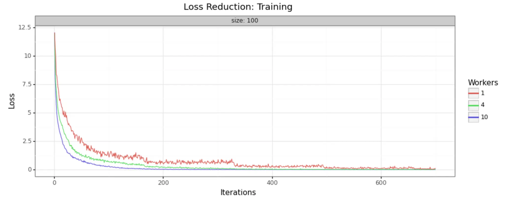
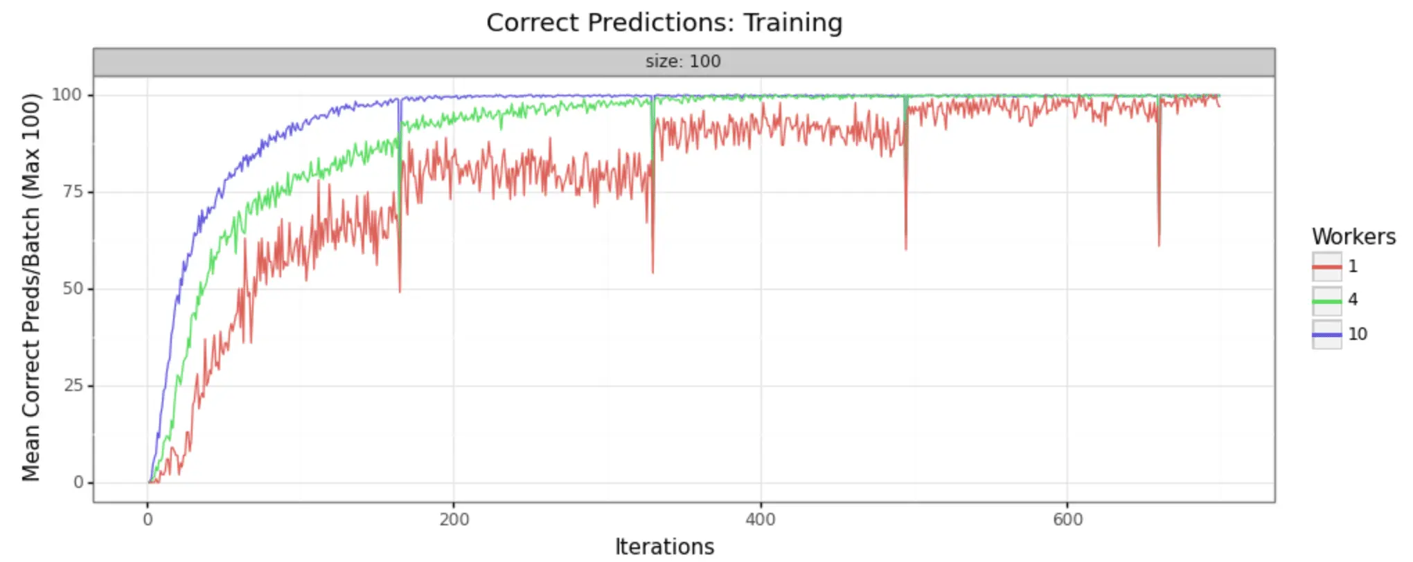
In order to demonstrate that this methodology is, in fact, producing improvements in model training, it can help to look at some visual representations of the statistics collected. We have run the job with three different sizes of cluster, to make it easy to see- 1 worker (single node), 4 workers, and 10 workers.
We can in fact see very noticeable performance gains in both loss reduction and accuracy. Batch size is 100 for each, and the adaptive learning rate begins at .01 for each. The train/test split is 80/20, as shown in the code above.
Training Samples
Evaluation Samples
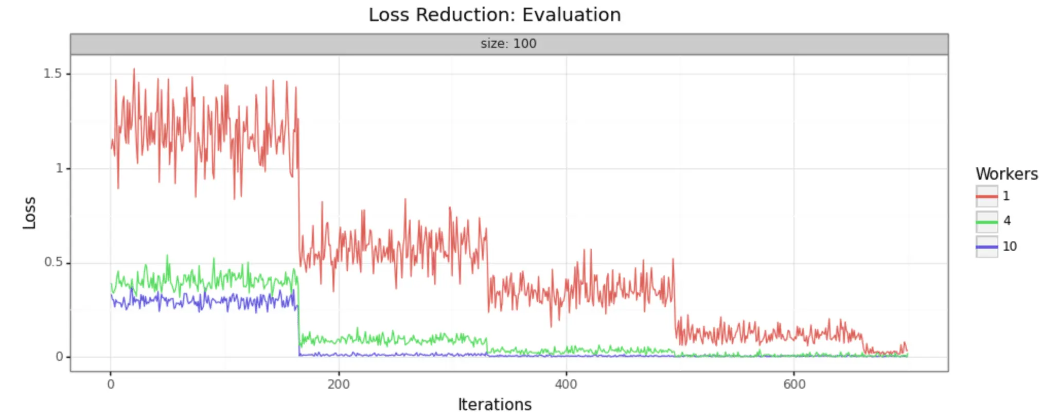
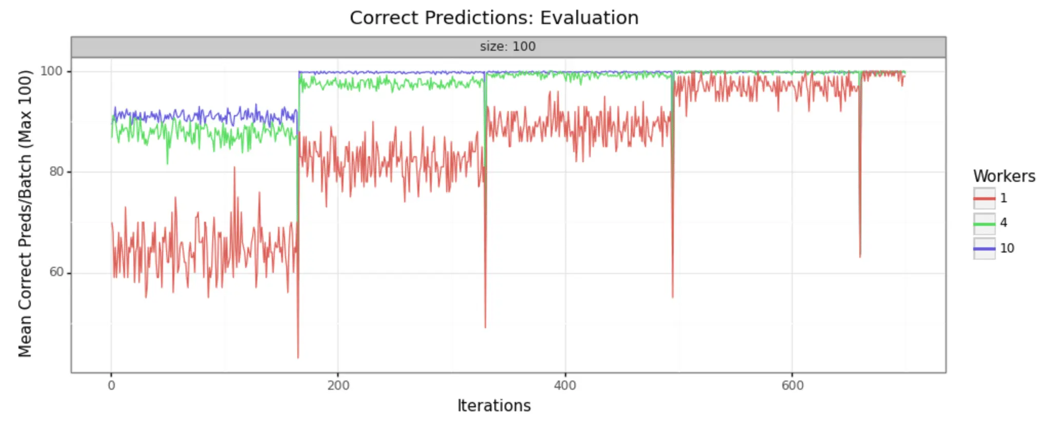
As you can see, increasing the number of workers in our cluster markedly improves the performance of training. In a 10-worker cluster, we reach peak performance around 200 iterations, while with the 4-worker cluster we must wait til 400 or more. In the single node example, at 600 we still have substantial noise in the loss value and may not reach the desired performance for many iterations to come.
Conclusion
It tremendously depends on the individual problem being solved, whether GPU clusters for transfer learning are the right choice, and some problems are not complex or challenging enough to call for this approach. However, for many deep learning problems, especially in the computer vision space, there can be a substantial value generated by using the increased computation resources and speeding up the achievement of ideal model performance.
For data scientists who would like to have faster, better performance on transfer learning and deep learning modeling tasks, we encourage you to give GPU clusters on Saturn Cloud a try! You can use our free version to experiment and see if this approach is right for your problem. Our plans allow individuals, teams, and enterprise to get started right away.
Thanks to Alvan Nee on Unsplash for the header image.
Additional Resources:
- Easily connect to Dask from outside of Saturn Cloud - This blog post walks through using a Saturn Cloud Dask cluster from a client outside of Saturn Cloud
- Saturn Cloud Dask examples - we have examples of using Dask for many different purposes, including machine learning and Dask with GPUs.
- Should I Use Dask?
- Easily Connect to Dask from Outside of Saturn Cloud
- [Lazy Evaluation with Dask](https://saturncloud.io/blog/a-data-scientist-s-guide-to-lazy-evaluation-with-dask/)
- Random Forest on GPUs: 2000x Faster than Apache Spark
- An Intro to Data Science Platforms
- What are Data Science Platforms
- Most Data Science Platforms are a Bad Idea
- Top 10 Data Science Platforms And Their Customer Reviews 2022
- Saturn Cloud: An Alternative to SageMaker
- PDF Saturn Cloud vs Amazon Sagemaker
- Configuring Sagemaker
- Top Computational Biology Platforms
- Top 10 ML Platforms
- What is dask and how does it work?
- Setting up JupyterHub
- Setting up JupyterHub Securely on AWS
- [Setting up HTTPS and SSL for JupyterHub](https://saturncloud.io/blog/securing-jupyterhub/)
- Using JupyterHub with a Private Container Registry
- Setting up JupyterHub with Single Sign-on (SSO) on AWS
- List: How to Setup Jupyter Notebooks on EC2
- [List: How to Set Up JupyterHub on AWS](https://saturncloud.io/blog/how-to-setup-jupyterhub-on-aws/)