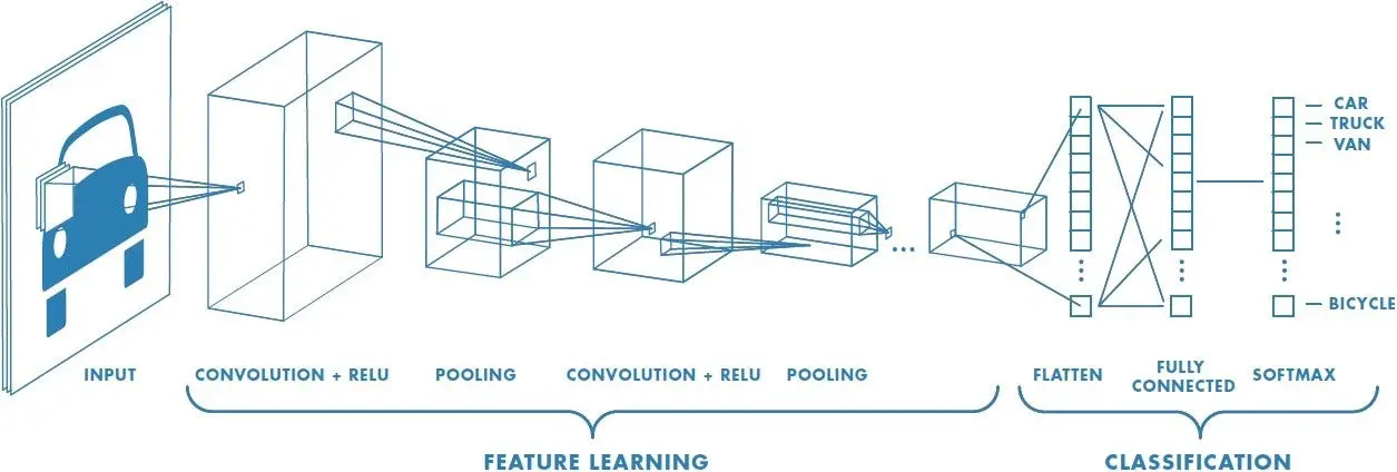
Artificial Intelligence has been witnessing monumental growth in bridging the gap between the capabilities of humans and machines. Researchers and enthusiasts alike, work on numerous aspects of the field to make amazing things happen. One of many such areas is the domain of Computer Vision.
The agenda for this field is to enable machines to view the world as humans do, perceive it in a similar manner, and even use the knowledge for a multitude of tasks such as Image & Video recognition, Image Analysis & Classification, Media Recreation, Recommendation Systems, Natural Language Processing, etc. The advancements in Computer Vision with Deep Learning have been constructed and perfected with time, primarily over one particular algorithm — a Convolutional Neural Network.

Introduction
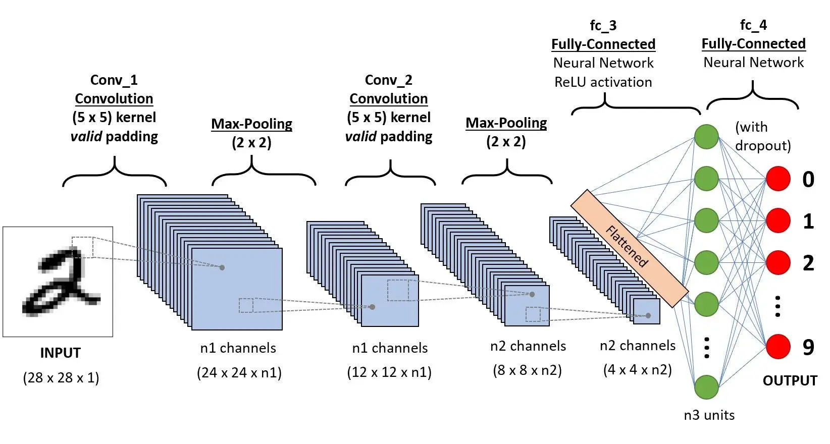
A CNN sequence to classify handwritten digits
A Convolutional Neural Network (ConvNet/CNN) is a Deep Learning algorithm that can take in an input image, assign importance (learnable weights and biases) to various aspects/objects in the image, and be able to differentiate one from the other. The pre-processing required in a ConvNet is much lower as compared to other classification algorithms. While in primitive methods filters are hand-engineered, with enough training, ConvNets have the ability to learn these filters/characteristics.
The architecture of a ConvNet is analogous to that of the connectivity pattern of Neurons in the Human Brain and was inspired by the organization of the Visual Cortex. Individual neurons respond to stimuli only in a restricted region of the visual field known as the Receptive Field. A collection of such fields overlap to cover the entire visual area.
Why ConvNets over Feed-Forward Neural Nets?
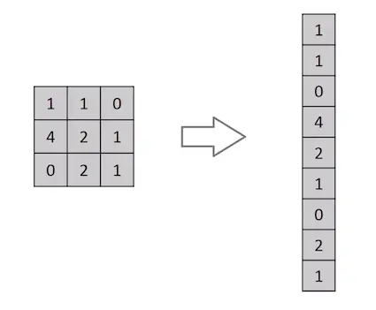
Flattening of a 3x3 image matrix into a 9x1 vector
An image is nothing but a matrix of pixel values, right? So why not just flatten the image (e.g. 3x3 image matrix into a 9x1 vector) and feed it to a Multi-Level Perceptron for classification purposes? Uh.. not really.
In cases of extremely basic binary images, the method might show an average precision score while performing prediction of classes but would have little to no accuracy when it comes to complex images having pixel dependencies throughout.
A ConvNet is able to successfully capture the Spatial and Temporal dependencies in an image through the application of relevant filters. The architecture performs a better fitting to the image dataset due to the reduction in the number of parameters involved and the reusability of weights. In other words, the network can be trained to understand the sophistication of the image better.
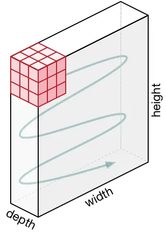
Input Image
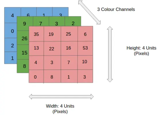
4x4x3 RGB Image
In the figure, we have an RGB image that has been separated by its three color planes — Red, Green, and Blue. There are a number of such color spaces in which images exist — Grayscale, RGB, HSV, CMYK, etc.
You can imagine how computationally intensive things would get once the images reach dimensions, say 8K (7680×4320). The role of ConvNet is to reduce the images into a form that is easier to process, without losing features that are critical for getting a good prediction. This is important when we are to design an architecture that is not only good at learning features but also scalable to massive datasets.
Convolution Layer — The Kernel
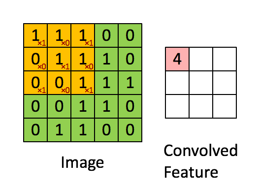
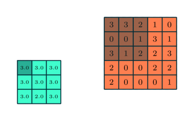
Convoluting a 5x5x1 image with a 3x3x1 kernel to get a 3x3x1 convolved feature
Image Dimensions = 5 (Height) x 5 (Breadth) x 1 (Number of channels, eg. RGB)
In the above demonstration, the green section resembles our 5x5x1 input image, I. The element involved in the convolution operation in the first part of a Convolutional Layer is called the Kernel/Filter, K, represented in color yellow. We have selected K as a 3x3x1 matrix.
    Kernel/Filter, K =

    1  0  1
    0  1  0
    1  0  1
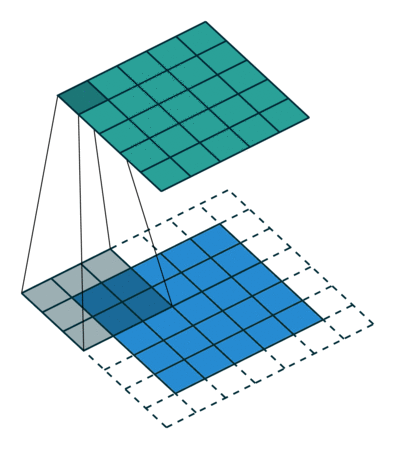
The Kernel shifts 9 times because of Stride Length = 1 (Non-Strided), every time performing an elementwise **multiplication operation (Hadamard Product) between K and the portion P of the image over which the kernel is hovering.
Movement of the Kernel
The filter moves to the right with a certain Stride Value till it parses the complete width. Moving on, it hops down to the beginning (left) of the image with the same Stride Value and repeats the process until the entire image is traversed.
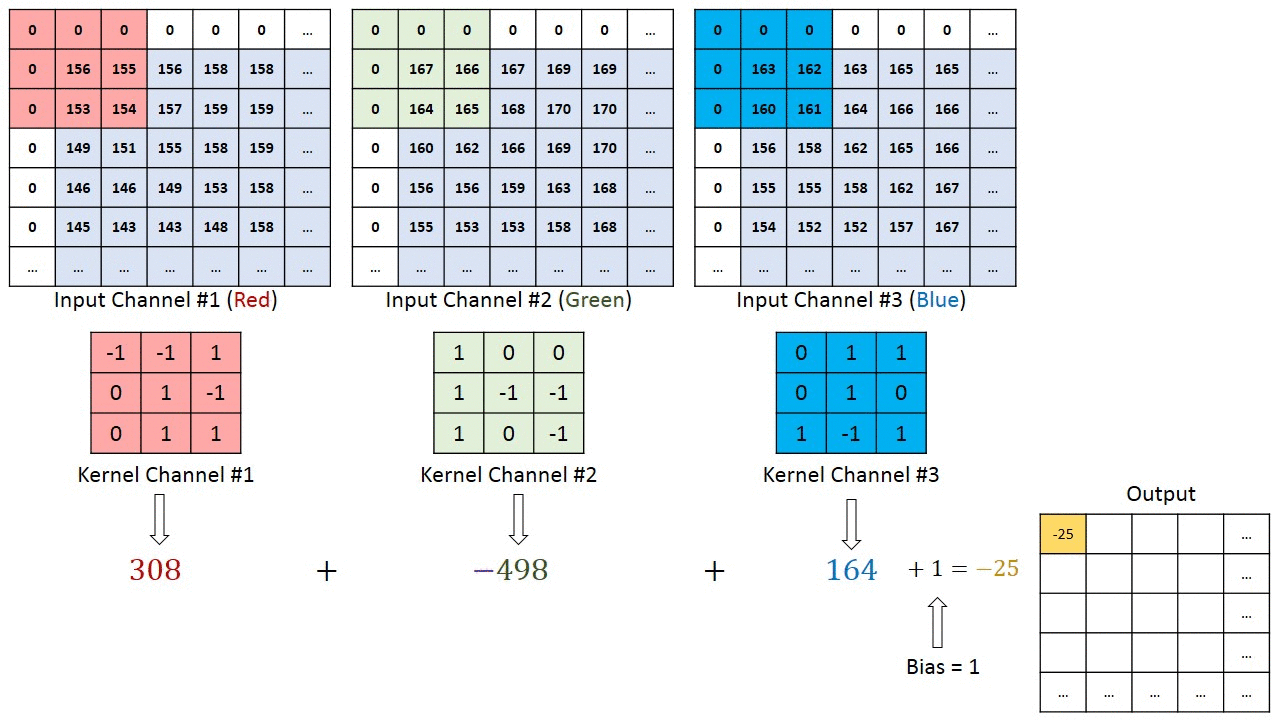
Convolution operation on a MxNx3 image matrix with a 3x3x3 Kernel
In the case of images with multiple channels (e.g. RGB), the Kernel has the same depth as that of the input image. Matrix Multiplication is performed between Kn and In stack ([K1, I1]; [K2, I2]; [K3, I3]) and all the results are summed with the bias to give us a squashed one-depth channel Convoluted Feature Output.
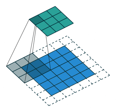
Convolution Operation with Stride Length = 2
The objective of the Convolution Operation is to extract the high-level features such as edges, from the input image. ConvNets need not be limited to only one Convolutional Layer. Conventionally, the first ConvLayer is responsible for capturing the Low-Level features such as edges, color, gradient orientation, etc. With added layers, the architecture adapts to the High-Level features as well, giving us a network that has a wholesome understanding of images in the dataset, similar to how we would.
There are two types of results to the operation — one in which the convolved feature is reduced in dimensionality as compared to the input, and the other in which the dimensionality is either increased or remains the same. This is done by applying Valid Padding in the case of the former, or Same Padding in the case of the latter.
When we augment the 5x5x1 image into a 6x6x1 image and then apply the 3x3x1 kernel over it, we find that the convolved matrix turns out to be of dimensions 5x5x1. Hence the name — Same Padding.
On the other hand, if we perform the same operation without padding, we are presented with a matrix that has dimensions of the Kernel (3x3x1) itself — Valid Padding.
The following repository houses many such GIFs which would help you get a better understanding of how Padding and Stride Length work together to achieve results relevant to our needs.
Pooling Layer
Similar to the Convolutional Layer, the Pooling layer is responsible for reducing the spatial size of the Convolved Feature. This is to decrease the computational power required to process the data through dimensionality reduction. Furthermore, it is useful for extracting dominant features which are rotational and positional invariant, thus maintaining the process of effectively training the model.
There are two types of Pooling: Max Pooling and Average Pooling. Max Pooling returns the maximum value from the portion of the image covered by the Kernel. On the other hand, Average Pooling returns the average of all the values from the portion of the image covered by the Kernel.
Max Pooling also performs as a Noise Suppressant. It discards the noisy activations altogether and also performs de-noising along with dimensionality reduction. On the other hand, Average Pooling simply performs dimensionality reduction as a noise-suppressing mechanism. Hence, we can say that Max Pooling performs a lot better than Average Pooling.
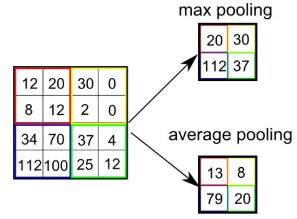
Types of Pooling
The Convolutional Layer and the Pooling Layer, together form the i-th layer of a Convolutional Neural Network. Depending on the complexities in the images, the number of such layers may be increased for capturing low-level details even further, but at the cost of more computational power.
After going through the above process, we have successfully enabled the model to understand the features. Moving on, we are going to flatten the final output and feed it to a regular Neural Network for classification purposes.
Classification — Fully Connected Layer (FC Layer)
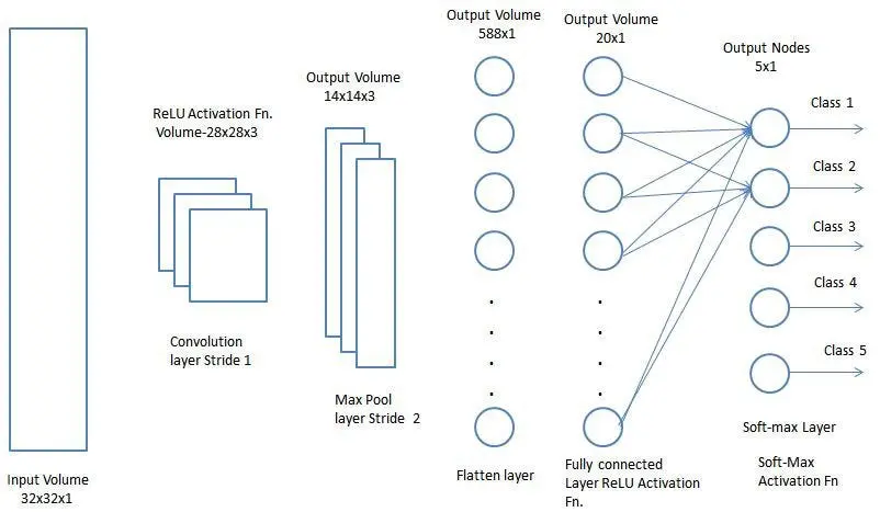
Adding a Fully-Connected layer is a (usually) cheap way of learning non-linear combinations of the high-level features as represented by the output of the convolutional layer. The Fully-Connected layer is learning a possibly non-linear function in that space.
Now that we have converted our input image into a suitable form for our Multi-Level Perceptron, we shall flatten the image into a column vector. The flattened output is fed to a feed-forward neural network and backpropagation is applied to every iteration of training. Over a series of epochs, the model is able to distinguish between dominating and certain low-level features in images and classify them using the Softmax Classification technique.
There are various architectures of CNNs available which have been key in building algorithms which power and shall power AI as a whole in the foreseeable future. Some of them have been listed below:
LeNet
AlexNet
VGGNet
GoogLeNet
ResNet
ZFNet
You may also be interested in:
- Speeding up Neural Network Training With Multiple GPUs and Dask
- Deep Learning with R
- Layer Pruning for Transformer Models
- Top 30 ML Tools for Foundation Models - 2023 Edition