Photo credit: ANIRUDH on Unsplash
Table of Content
- Introduction
- Transformer and various ways to shrink transformer model
- What is pruning
- Types of pruning and its use cases
- Let’s prune a pre-train model to reduce the inference latency
Introduction:
As the demand and applications for large language model become popular and impressive, the development of models becomes important as well. One of the most notable advancements in recent years in the machine learning ecosystem is the Transformer models, which have set new performance benchmarks across various NLP tasks like translation, chatbot (ChatGPT, dialogflow etc), classification and computer vision. While these models have a great impact, their large size and computational prerequisites become a challenge for deployment in real-world applications (cloud, or edge deployment), particularly in limited resource environments or scenarios where low-latency is a priority.
One interesting approach to solve these challenges is pruning, a technique that aims to reduce the size and complexity of Transformer models without significantly affecting their performance.
In this article, we will explore the concept of layer pruning, and provide practical examples of how it can be applied to Transformer models (XLM-RoBERTa)
Transformer:
In today’s AI revolution, Transformer architecture is the bedrock of amazing AI tools that have been released in the past few months. we have alot of amazing models released by open AI, like GPT (GPT3.5, GPT4) and other amazing models.
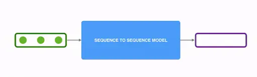
Transformer is a type of neural network architecture that has gained fame over RNNs and LSTM on NLP tasks like translation, and sequence-to-sequence tasks(basically any task that involves an input sequence to an output sequence). It outperforms seq-to-seq models by capturing the vital context in the text.
For example “Bill bought Oreos and salad. He also paid in cash” in the first sentence, “Bill” bought Oreos but the second sentence refers that Bill paid for xyz item in cash. When you read the first sentence and the second, you do refer to the word in the first sentence right?
With the example above, for a model to achieve sequence transduction it is necessary for the model to have some memory to recall the previous sentences.
Before Transformer, we had RNNs (Recurrent Neural networks) and LSTM (Long short term memory); these architectures were focused on sequential processing but word-by-word and past information is retained through gates or hidden state.
Some of the characteristics of RNNs where transformers perform better include:
Parallelization: Transformers can process all positions in a sequence in parallel, which makes them much faster than RNNs and sentences are processed in full instead of word by word.
Memory efficiency: RNNs need to store the hidden state for each position in a sequence, which makes them memory-intensive. In contrast, Transformers only need to store the embeddings for each position in a sequence, which makes them more memory-efficient.
Positional embeddings: Positional encoding in Transformer is another innovative characteristic. The idea of positional embedding is basically used to fix or learned weights which encode information related to a specific position of a token in a sentence.
How Transformer works:
Transformers basically use attention mechanisms to solve problems without recurrence and are faster to train. The attention mechanism in the transformer allows it to pay attention to the important context in a text or corpus. In a nutshell, we can compute the attention of a sequence by first calculating a set of attention weights for each word in the sequence. These weights represent the relevance of each word to the other words in the sequence.
Let’s use our example in the previous section “Bill bought Oreos and salad. He also paid in cash” and let’s say we want to compute for the attention of this sentence, first we split the token into a sequence of token below;
[“Bill”, “bought”, “Oreos”, “and”, “salad”, “.”, “He”, “also”, “paid”, “in”, “cash”, “."]
Then, compute the set of query, key and value vector for each token. The query vector for each token represents the token, on the hand, the value and key vector represent the other token in the sequence
For example, the query vector for the token “Bill” would be derived from the word embedding for “Bill”, while the key and value vectors would be derived from the embeddings for all the other tokens in the sequence.
Once the query, key, and value vectors have been computed, the Transformer computes a set of attention weights for each token. These weights represent how much attention the model should pay to each of the other tokens in the sequence when processing the current token. For example, when processing the token “Bill”, the model might assign high attention weights to the tokens “bought”, “Oreos”, and “salad”, which are all related to the action of buying groceries.
Additionally, transformer models have encoders and decoders components.
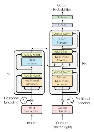
The encoder (left side) has one attention head and a feedforward neural network layer. The encoder takes in input sequence, which is typically a sequence of tokens representing words or subwords in a sentence, and produces a set of hidden representations that capture the meaning of each token in the sequence, on the other hand, decoders(right side) have two attention head and one feed forward neural network. The decoder uses the encoder result or embeddings along with its input to generate the expected result or sequence
One of the drawbacks of transformer large language models is high latency. Now that we have an idea about transformers and how it works, let’s look at how we can optimize the attention head via pruning in order to optimize the latency.
Pruning: From the above diagram we can see that there are three kinds of attention heads in transformer architecture,
- Multi head attention
- Masked Multi head attention
- Multi head attention encoder decoder
Layer pruning is a technique used to reduce the latency and computation cost of transformer models by removing redundant layers or heads while maintaining performance. The goal of pruning is to find an optimal trade-off between model complexity and performance, making the model more efficient and easier to deploy.
Layer pruning can be performed through various methods, such as weight pruning, neuron pruning, attention head pruning, greedy pruning.
Weight pruning:
Weight pruning: In weight pruning, the smallest weights (based on their absolute values) in the model are removed or set to zero. This reduces the number of non-zero weights and thus the overall complexity of the model. Weight pruning can be performed at different levels of granularity, such as individual weights, weight matrices, or weight tensors.
Neuron Pruning:
Neuron pruning: Neuron pruning involves removing neurons (or hidden units) from the model’s layers. This can be done based on the importance of the neuron, which is typically measured by the magnitude of its activation or its contribution to the final output. By removing less important neurons, the model’s complexity is reduced while keeping the most relevant features intact.
Greedy-layer pruning:
Greedy layer pruning is said to be a state of the art pruning technique that put perform knowledge distillation by repeating the steps of head importance scoring, layer elimination, and fine-tuning iteratively until you reach the desired number of layers or excellent performance level. This process is called greedy because, at each iteration, you are only removing one layer and then fine-tuning the model, rather than eliminating multiple layers at once.
Read more: https://deepai.org/publication/greedy-layer-pruning-decreasing-inference-time-of-transformer-models
Attention head pruning: Attention head pruning is a specific type of pruning technique used in transformer models. It doesn’t fall directly under weight pruning or neuron pruning, but it is somewhat related to both.
In this sense, attention head pruning can be seen as a combination of weight and neuron pruning. By removing an attention head, you are effectively pruning the weights associated with that head and also the neurons responsible for computing the attention scores and context vectors within that head.
The goal of attention head pruning is to reduce the complexity of the transformer model while maintaining its performance. By identifying and removing less important or redundant attention heads, you can create a smaller and more computationally efficient model that still achieves good results.
Now we have a clear understanding of layer pruning and various type, lets jump into a more practical step on pruning XLM-RoBERTa Model
Prune a pretrain models to reduce the inference latency
Requirements:
Step 1: Load the pretrain model
In this step, we will load xlm-Roberta-base model via hugging face
import textpruner
from transformers import XLMRobertaForSequenceClassification,XLMRobertaTokenizer

from textpruner import summary, TransformerPruner
import sys

from transformers import AutoTokenizer, AutoModelForMaskedLM,XLMModel

tokenizer = AutoTokenizer.from_pretrained("xlm-roberta-base")

model = AutoModelForMaskedLM.from_pretrained("xlm-roberta-base")
Step 2: visualize the number of attention heads
In this step we will visulize the number of attention heads and check for heads importance so we can in the next step eliminate head with low importance to the model performance
from transformers import AutoTokenizer, AutoModel, utils
from bertviz import model_view, head_view
utils.logging.set_verbosity_error()

inputs = tokenizer.encode("The cat sat on the mat", return_tensors='pt')
outputs = model(inputs)
attention = outputs[-1]  # Output includes attention weights when output_attentions=True
tokens = tokenizer.convert_ids_to_tokens(inputs[0])

from bertviz import head_view
model_view(attention, tokens)
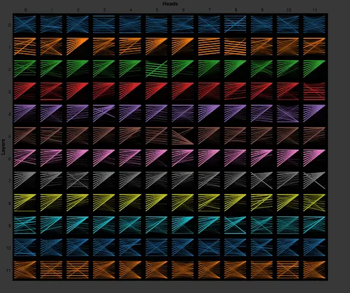
The chart above visualize the attention mechanism in the XLM-RoBERTa model and it provides an interactive representation of the attention scores for each attention head in the model’s layers. Additionally, the attention heads is a core component of Transformer models
The chart has the following components:
Layers: The X-axis display the layers of the model, which are stacked on top of each other. Each layer is responsible for capturing different levels of abstraction in the input text. In XLM-RoBERTa-base, there are 12 layers.
Heads: The Y-axis display the attention heads within each layer and each layer in XLM-RoBERTa-base has 12 attention heads.
The chart also hover the follow components:
Tokens: The input sentence tokens are displayed on both the left and right sides of the chart. The left-side tokens are the “query” tokens, while the right-side tokens are the “key” tokens.
Attention Scores: The lines connecting the “query” tokens to the “key” tokens represent the attention scores. The thickness of the lines indicates the strength of the attention score between the corresponding tokens. A thicker the line, the higher attention score, meanwhich means that the model is paying more attention to the relationship between those two tokens. This can help identify which words in the sentence the model considers relevant or important with respect to each other.
Step 3: Prune the model and evaluate inference time using text pruner
print("Before pruning:")
print(summary(model))


pruner = TransformerPruner(model)

ffn_mask = textpruner.pruners.utils.random_mask_tensor((12,3072))
head_mask = textpruner.pruners.utils.random_mask_tensor((12,12), even_masks=False)

pruner.prune(head_mask=head_mask, ffn_mask=ffn_mask,save_model=True)

print("After pruning:")
print(summary(model))

for i in range(12):
    print ((model.base_model.encoder.layer[i].intermediate.dense.weight.shape,
            model.base_model.encoder.layer[i].intermediate.dense.bias.shape,
            model.base_model.encoder.layer[i].attention.self.key.weight.shape))


token =tokenizer("Hello, i am looking <mask> Jammie",return_tensors="pt")

# model.device("cpu")
inference = textpruner.inference_time(model,token)
print(inference)
The code above print model summary before pruning first using the summary() function from the textpruner library which is used to print the model’s architecture and the number of parameters before pruning.
Second, we Initialize the TransformerPruner, which creates a TransformerPruner object, which is used to prune the model.
Third, we create random head and ffn(feed forward network) masks using the random_mask_tensor function from the TextPruner library. The ffn mask and random head masks are used to selectively prune the feed-forward network (FFN) and attention heads of the pre-trained XLM-Roberta model, respectively. The need for pruning these components of the model is to reduce the computational and memory requirements of the model, while maintaining or even improving its performance.
Next, we prune the model using prune() method of the TransformerPruner object with the generated head_mask and ffn_mask. This method prunes the model by eliminating the attention heads and FFN layers specified by the masks, then we use the save_model parameter is set to True, which means the pruning will be saved in our directory
Last, we use the summary() function again to print the model’s architecture and the number of parameters after pruning and then, we tokenize a sample sentence with a masked token and feeds the tokens into the pruned model for inference. The textpruner.inference_time(model,token) function measures the time taken to perform the inference.
Additionally, the steps above can be applied to a fine-tuned transformer model. After fine-tuning you can apply the pruning steps process and as well perform quantization using Onnx. Last, you can perform benchmarking between inference without pruning and inference after pruning.
You may also be interested in:
Greedy Layer Pruning: Decreasing Inference Time of Transformer Models
[BertViz: Visualize Attention in NLP Models (BERT, GPT2, BART, etc.)](https://github.com/jessevig/bertviz)
Knowledge Distillation: Principles, Algorithms, Applications