
This article was published when data science tooling like Dask and R was a primary focus for Saturn Cloud. Today, Saturn Cloud is the enterprise AI platform for any GPU infrastructure.
As a data scientist, one of the most common tasks you’ll encounter is reading data from CSV files. These files are widely used to store tabular data, and they can be easily created and manipulated using spreadsheet software like Microsoft Excel or Google Sheets. However, when working with large datasets, it’s often more convenient to use a programming language like Python and a tool like Jupyter Notebook. You can use Jupyter notebooks for free online at Saturn Cloud.
Jupyter Notebook is an open-source web application that allows you to create and share documents containing live code, equations, visualizations, and narrative text. It supports many programming languages, including Python, R, and Julia, and it’s widely used in data science, scientific research, and education.
Struggling with reading CSV files in Jupyter Notebook online? Simplify your data science tasks with Saturn Cloud. Begin your free trial today and experience seamless file handling!
In this tutorial, we’ll show you how to read a CSV file in Jupyter Notebook online using Python and the Pandas library. Pandas is a powerful data manipulation library that provides easy-to-use data structures and data analysis tools for Python.
Step 1: Import the Pandas library
To use the Pandas library, you need to import it into your Jupyter Notebook. You can do this by running the following command:
import pandas as pd
This command imports the Pandas library and assigns it the alias “pd”, which is a common convention in the Python community.
Step 2: Load the CSV file
To load a CSV file into Pandas, you can use the read_csv() function. This function takes the path to the CSV file as a parameter and returns a DataFrame object, which is a two-dimensional table-like data structure that can hold data of different types.
Assuming that your CSV file is stored in the same directory as your Jupyter Notebook, you can load it by running the following command:
df = pd.read_csv('data.csv')
This command reads the CSV file named “mydata.csv” and stores its contents in a DataFrame object named “df”. You can replace “data.csv” with the name of your CSV file.
If your CSV file is stored in a different directory, you need to provide the full path to the file. For example, if your CSV file is stored in the “data” directory of your Jupyter Notebook, you can load it by running the following command:
df = pd.read_csv('data/mydata.csv')
This command reads the CSV file named data.csv from the “data” directory and stores its contents in a DataFrame object named df.
Step 3: Explore the data
Once you’ve loaded the CSV file into a DataFrame object, you can start exploring its contents. Pandas provides many functions and methods for data manipulation, aggregation, and visualization.
For example, you can use the head() function to display the first five rows of the DataFrame:
df.head()
Output:
      col1 col2 col3 col4
0        x   15    a   20
1        y   16    b   18
2        x   17    c   16
3        y   18    d   14
4        x   19    e   12
This command displays the first five rows of the DataFrame. You can change the number of rows displayed by passing a parameter to the head() function. For example, to display the first three rows, you can run:
df.head(3)
Output:
      col1 col2 col3 col4
0        x   15    a   20
1        y   16    b   18
2        x   17    c   16
You can also use the describe() function to get a statistical summary of the DataFrame:
df.describe()
Output:
	    col2	col4
count	    6.000000	6.000000
mean	    17.500000	15.000000
std	    1.870829	3.741657
min	    15.000000	10.000000
25%	    16.250000	12.500000
50%	    17.500000	15.000000
75%	    18.750000	17.500000
max	    20.000000	20.000000
This command displays the count, mean, standard deviation, minimum, and maximum values for each column of the DataFrame. If your DataFrame contains non-numeric columns, the describe() function will skip them.
Step 4: Manipulate the data
Pandas provides many functions and methods for manipulating the data in a DataFrame. For example, you can drop, add a column or a row, rename column’s names, replace values in Dataframe, and many other operations.
df_drop = df.drop("col3", axis = 1)
print(df_drop)
This command drops the col3 of the Dataframe.
Output:
      col1 col2 col4
0        x   15    20
1        y   16    18
2        x   17    16
3        y   18    14
4        x   19    12
5        x   20    10
col5 = ["foo", "bar", "foo", "bar", "foo", "bar"]
df_add = df.assign(col5 = col5)
print(df_add)
This command adds a new column named col5 to the right of the Dataframe.
Output:
      col1 col2 col3 col4  col5
0        x   15    a   20   foo
1        y   16    b   18   bar
2        x   17    c   16   foo
3        y   18    d   14   bar
4        x   19    e   12   foo
5        x   20    f    10  bar
df_rename = df.copy()
df_rename.columns = ["x1", "x2", "x3", "x4"]
print(df_rename)
This command renames the columns of the Dataframe from col1, col2, col3, col4 to x1, x2, x3, x4.
Output:
        x1   x2   x3   x4
0        x   15    a   20
1        y   16    b   18
2        x   17    c   16
3        y   18    d   14
4        x   19    e   12
5        x   20    f   10
new_row = ["a", "b", "c", "d"]
df_new = df.copy()
df_new.loc[6] = new_row
print(df_new)
This command adds a new row to the bottom of the Dataframe.
Output:
      col1 col2 col3 col4
0        x   15    a   20
1        y   16    b   18
2        x   17    c   16
3        y   18    d   14
4        x   19    e   12
5        x   20    f   10
6        a    b    c    d
df_replace = df.copy()
df_replace["col1"] = df_replace["col1"].replace("y", "foo")
print(df_replace)
This command replaces any values y in col1 with foo.
Output:
      col1 col2 col3 col4
0        x   15    a   20
1      foo   16    b   18
2        x   17    c   16
3      foo   18    d   14
4        x   19    e   12
5        x   20    f   10
Step 5: Visualize the data
Pandas provides many functions and methods for visualizing the data in a DataFrame. For example, you can use the plot() function to create a line plot of a column:
df['col2'].plot()
Output:
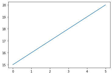
This command creates a line plot of the column named col2. You can replace col2 with the name of your column.
You can also use the scatter() function to create a scatter plot of two columns:
df.plot.scatter(x='col2', y='col4')
Output:
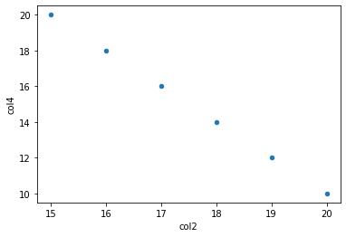
This command creates a scatter plot of the columns named col2 and col4. You can replace col2 and col4 with the names of your columns.
Struggling with reading CSV files in Jupyter Notebook online? Simplify your data science tasks with Saturn Cloud. Begin your free trial today and experience seamless file handling!
Conclusion
In this tutorial, we’ve shown you how to read a CSV file in Jupyter Notebook online using Python and the Pandas library. We’ve covered the basic steps of importing the Pandas library, loading the CSV file, exploring the data, manipulating the data, and visualizing the data.
We hope that this tutorial has been helpful to you and that you’re now ready to start working with CSV files in Jupyter Notebook.