PyTorch for Natural Language Processing: Building a Fake News Classification Model
Source
The proliferation of fake news has become a pressing concern in today’s digital age. To attempt to combat the spread of misinformation, you need effective tools and techniques. Specifically, Natural Language Processing (NLP) techniques help you extract meaning from vast amounts of text data, which can solve the issue of misinformation.
In this article, we explore the power of PyTorch, a popular deep-learning framework, in building a fake news classification model.
What’s PyTorch?
PyTorch provides a rich ecosystem of tools and libraries for constructing sophisticated neural network models. By leveraging PyTorch’s capabilities, you can develop classifiers for NLP tasks, in this case, a model that distinguishes between real and fake news.
Whether you are an NLP enthusiast, a data scientist, or a developer interested in applying deep learning to real-world problems, this article will teach you how to build a fake news classification model with PyTorch.
Let’s delve in!
Dependencies
In this tutorial, we used the Python programming language. The following libraries were used:
- Pandas: A powerful data manipulation and analysis library for Python.
- NumPy: A fundamental package for scientific computing with Python, supporting large, multi-dimensional arrays and mathematical functions.
- Requests: A Python library for making HTTP requests and handling responses simply and elegantly.
- Seaborn: A data visualization library based on Matplotlib, providing a high-level interface for creating informative and attractive statistical graphics.
- Matplotlib: A comprehensive plotting library for Python, offering various visualizations for exploring and presenting data.
- NLTK (Natural Language Toolkit): A library for natural language processing, providing tools and resources for tasks such as tokenization, stemming, tagging, and parsing.
- Transformers: A library built on the PyTorch framework, offering state-of-the-art models and methods for natural language understanding and generation tasks. The Bidirectional Encoder Representations from Transformers (BERT) model will be utilized in this tutorial via transfer learning.
- Scikit-learn: A versatile machine learning library for Python, providing efficient tools for data preprocessing, model selection, and evaluation.
- Newspaper: A Python library for article scraping and extraction, allowing easy retrieval of news articles and relevant information from online sources.
- Datasets: A library that provides access to various pre-built datasets for machine learning and data analysis tasks.
- Wordcloud: A library for generating word clouds, which are visual representations of text data where the size of each word reflects its frequency or importance in the text.
You can find the full code for this demo in this Colab notebook.
Import necessary libraries and modules
import pandas as pd
import numpy as np
import requests
import seaborn as sns
import matplotlib.pyplot as plt
import nltk

from transformers import BertTokenizer, BertForSequenceClassification
from torch.utils.data import TensorDataset, DataLoader

nltk.download('stopwords')
nltk.download('punkt')
To leverage Colab’s free GPU, please refer to the provided instructions for setup. It’s worth noting that some libraries mentioned in this tutorial might not be pre-installed in your Colab environment. Therefore, you may need to install them manually to ensure their availability.
Now that you are all set up, let’s load the data!
Loading and Cleaning Data
The dataset used in this tutorial was obtained from Huggingface’s dataset directory. You can download it programmatically with the following code:
from datasets import load_dataset

# loads the "fake_news_english" dataset from Huggingface
dataset = load_dataset("fake_news_english")
train_data = dataset["train"]
To view the data you have loaded, which is in dictionary format, convert the training data to a dataframe using the pandas library. This conversion will allow you to explore and analyze the data conveniently.
## converts training dataset into a dataframe
df = pd.DataFrame.from_dict(dataset['train'])

df.head()
When you explore the dataset, you can gain valuable insights into its features. This exploration helps you understand the nature of the data and determine the necessary transformations or preprocessing steps you can use to work with it effectively.
print(df.info())
print(df.describe())
print(df.shape)
Output (DO NOT COPY):
<class 'pandas.core.frame.DataFrame'>
RangeIndex: 492 entries, 0 to 491
Data columns (total 4 columns):
 #   Column                    Non-Null Count  Dtype
---  ------                    --------------  -----
 0   article_number            492 non-null    int64
 1   url_of_article            492 non-null    object
 2   fake_or_satire            492 non-null    int64
 3   url_of_rebutting_article  492 non-null    object
dtypes: int64(2), object(2)
memory usage : 15.5+ KB
None    article_number  fake_or_satire
count      492.000000      492.000000
mean       289.792683        0.591463
std        169.817410        0.492064
min          2.000000        0.000000
25%        138.750000        0.000000
50%        296.500000        1.000000
75%        432.250000        1.000000
max        595.000000        1.000000
(492, 4)
Inspecting the dataset columns, you’ll realize that the texts for the articles are not provided. The URLs to the articles are the only things you are given to work with. To transform this dataset into something you can work with, the URLs need to be scraped to get the body of text they contain.
To do this, you can create a function that scrapes content from a site and saves it in a new dataframe:
## loops through URLs in dataframe
  for url in df[column_name]:
      try:
          ## creates Article object and download/parse HTML content
          article = Article(url)
          article.download()
          article.parse()

          ## extracts title and main article text using newspaper3k
          title = article.title
          text = article.text

          ## appends extracted data to lists
          title_list.append(title)
          text_list.append(text)

      ## checks for specific types of exceptions that may be raised
      except requests.exceptions.HTTPError as errh:
        print("HTTP Error:", errh)
      except requests.exceptions.ConnectionError as errc:
          print("Error Connecting:", errc)
      except requests.exceptions.Timeout as errt:
          print("Timeout Error:", errt)
      except requests.exceptions.RequestException as err:
          print("Something went wrong:", err)
      except:
          print("An error occurred while processing the URL:", url)

  # creates new dataframe with scraped data
  new_df = pd.DataFrame({'title': title_list, 'text': text_list})
  new_df = new_df['title']+new_df['text']

  return new_df
Implement the function in your dataset:
## implementing 'scrape_website' function
df['text'] = scrape_website(df, 'url_of_article')
Output (DO NOT COPY):
An error occurred while processing the URL: http://president45donaldtrump.com/breaking-study-proves-trump-right-every-citizen-voter-betrayed/
An error occurred while processing the URL: http://president45donaldtrump.com/0-23-0/
An error occurred while processing the URL: http://president45donaldtrump.com/1-9892-2/
An error occurred while processing the URL: http://24wpn.com/index.php/2017/04/29/hillary-clinton-busted-in-the-middle-of-huge-pedophilia-ring-cover-up-at-state-department-video/
An error occurred while processing the URL: http://24wpn.com/index.php/2017/04/29/breaking-sharia-law-is-gone-the-house-made-a-decision/
An error occurred while processing the URL: http://24wpn.com/index.php/2017/08/21/breaking-wasserman-schultz-aide-imran-awan-under-investigation-for-allegedly-selling-secrets-to-russians/

...
The output reveals that certain URLs in the URL column are non-functional and irrelevant to the dataset. To address this, the function selectively retains the content from the operational sites and stores it in a new column.
You can clean your dataset a little to prepare it for analysis and modeling by renaming columns, dropping duplicates, and removing irrelevant columns.
## renames columns, drop duplicates and unwanted columns
df.rename(columns = {'fake_or_satire': 'labels'}, inplace = True)
df = df.drop_duplicates('text', keep=False)
df = df.drop(['article_number', 'url_of_article', 'url_of_rebutting_article'], axis = 1)

df ## displays dataframe
Output (DO NOT COPY):
The cleaned dataset:

labels	                                             text
24	1	A Russian Writer Claiming To Be Putin's Lover ...
25	1	Clinton's assistant J. W. McGill is found dead...
34	1	Roger Stone Blames Obama For The Possibility O...
35	1	Bill O'Reilly: "Companies Under Trump Must Say...
37	1	Proof that Mass Voter Fraud Swung New Hampshir...
...	...	...
299	0	Trump to Nominate Chris Christie to Supreme Fo...
300	0	Trump to Limit All Intelligence Briefings to 1...
301	0	Obama to Send Large Shipment of 'Thoughts and ...
302	0	Trump: Ben Carson Perfect For HUD Because 'It ...
303	0	Why Won't You Just Let Us Pass a Health Care B...
196 rows × 2 columns
Data Exploration After loading and cleaning the data, you need to check if the dataset set is balanced and understand elements like the label distribution, distribution of text length, and frequency of words in both fake news and true news.
## displays information about the different labels
df[df['labels'] == 0].info()
df[df['labels'] == 1].info()
Output (DO NOT COPY):
<class 'pandas.core.frame.DataFrame'>
Int64Index: 13 entries, 291 to 303
Data columns (total 2 columns):
 #   Column  Non-Null Count  Dtype
---  ------  --------------  -----
 0   labels  13 non-null     int64
 1   text    13 non-null     object
dtypes: int64(1), object(1)
memory usage: 312.0+ bytes
<class 'pandas.core.frame.DataFrame'>
Int64Index: 183 entries, 24 to 290
Data columns (total 2 columns):
 #   Column  Non-Null Count  Dtype
---  ------  --------------  -----
 0   labels  183 non-null    int64
 1   text    183 non-null    object
dtypes: int64(1), object(1)
memory usage: 4.3+ KB
The following code provides a visual representation of the distribution between true and fake news in the dataset:
## shows the distribution of labels on a bar chart
sns.countplot(y='labels', palette="coolwarm", data=df).set_title('Distribution of true or fake news')
plt.show()

As you can see, the data is unbalanced.
1 = Fake News 0= True News.
This is typical for most real-world data. You have to decide what to do. Here are some options:
One approach is to augment the dataset by adding more samples from the minority class or balancing the class distribution overall. This can involve collecting more data with labels from the underrepresented class or employing techniques like Synthetic Minority Over-sampling Technique (SMOTE) to generate synthetic samples.
For text data, you can apply techniques like oversampling and undersampling specifically to the text samples. This involves replicating or removing text samples to balance the class distribution. Specialized libraries like imbalanced-learn provide methods like SMOTE or TomekLinks for text data.
Note that in this tutorial, those techniques are not covered.
Analyzing the distribution of prominent words in your dataset is valuable for understanding the association between specific words and fake or true news. A word cloud serves as an effective tool to visualize this information.
## the following code generates a word cloud

## filters data for fake and true news
fake_news = df[df['labels'] == 1]
true_news = df[df['labels'] == 0]

## concatenates all text for each category
fake_text = ' '.join(fake_news['text'].tolist())
true_text = ' '.join(true_news['text'].tolist())

## sets stopwords for text preprocessing
stop_words = set(stopwords.words('english'))

## generate word clouds for each category
fake_wordcloud = WordCloud(stopwords=stop_words, background_color='white').generate(fake_text)
true_wordcloud = WordCloud(stopwords=stop_words, background_color='white').generate(true_text)

## plots the word clouds
fig, axs = plt.subplots(1, 2, figsize=(20, 10))
axs[0].imshow(fake_wordcloud, interpolation='bilinear')
axs[0].set_title('Fake News')
axs[0].axis('off')
axs[1].imshow(true_wordcloud, interpolation='bilinear')
axs[1].set_title('True News')
axs[1].axis('off')
plt.show()
Output (DO NOT COPY):

It is also great to understand some descriptive statistics on the text dataset, like the number of news texts you have, the maximum, and the mean text length.
The number of news texts in the dataset gives us an understanding of the size and volume of the data. This information helps gauge the dataset’s scale and potential for analysis and modeling.
The maximum text length refers to the longest news text in the dataset. It helps identify the text’s complexity and provides insights into the potential challenges of processing or analyzing longer texts.
Calculating the mean length of the news texts provides an average measure representing the typical text length in the dataset. This statistic allows us to understand the overall length distribution and helps determine the appropriate preprocessing or modeling techniques to apply:
words = [text for text in df.text]

max_len = 0
text_len = []

## loops through text data to get the max_len and mean length
for texts in words:
  text_len.append(len(texts.split())) ## calculates and appends to text_len
  max_len = max(len(texts.split()), max_len) ## updates max_len

## displays results
print('Number of news text:', len(words))
print('Max length of the text:', max_len)
print('Mean length of the text:', np.mean(text_len))
Output (DO NOT COPY):
Number of news text: 196
Max length of the text: 3602
Mean length of the text: 425.4030612244898
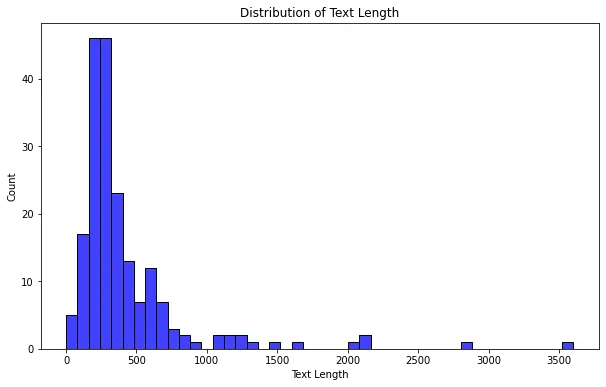
Checking the distribution of text length in a dataset serves several purposes. Firstly, it provides insights into the variability of text lengths within the dataset. Understanding the range and spread of text lengths helps determine appropriate preprocessing steps, such as setting maximum sequence lengths for models or applying padding techniques.
Additionally, analyzing the distribution of text length can uncover patterns or anomalies that impact downstream tasks. For instance, it can reveal the presence of unusually long texts requiring special handling or highlight the prevalence of shorter texts requiring different modeling approaches. By examining the distribution of text length, researchers and practitioners can make informed decisions regarding data preprocessing, model selection, and optimization to ensure the best possible outcomes for natural language processing tasks.
## plots the distribution of text lengths
plt.figure(figsize=(10, 6))
sns.histplot(text_len, kde=False, color='blue')

## sets the axis labels and title
plt.xlabel('Text Length')
plt.ylabel('Count')
plt.title('Distribution of Text Length')

## displays the plot
plt.show()
Output (DO NOT COPY):
Save the dataset to your drive so you do not have to repeat all these processes and access it easily if anything happens to your Colab session.
## converts dataframe to CSV

from google.colab import drive
drive.mount('/content/drive')

## Specify the directory you want to read the data from
dir = "/content/drive/My Drive/"

df.to_csv(f'{dir}/fake_news_english.csv')
BERT Model
BERT (Bidirectional Encoder Representations from Transformers) is a pre-trained language model developed by Google. It revolutionized the field of natural language processing (NLP) by introducing a novel approach to learning contextualized word representations.
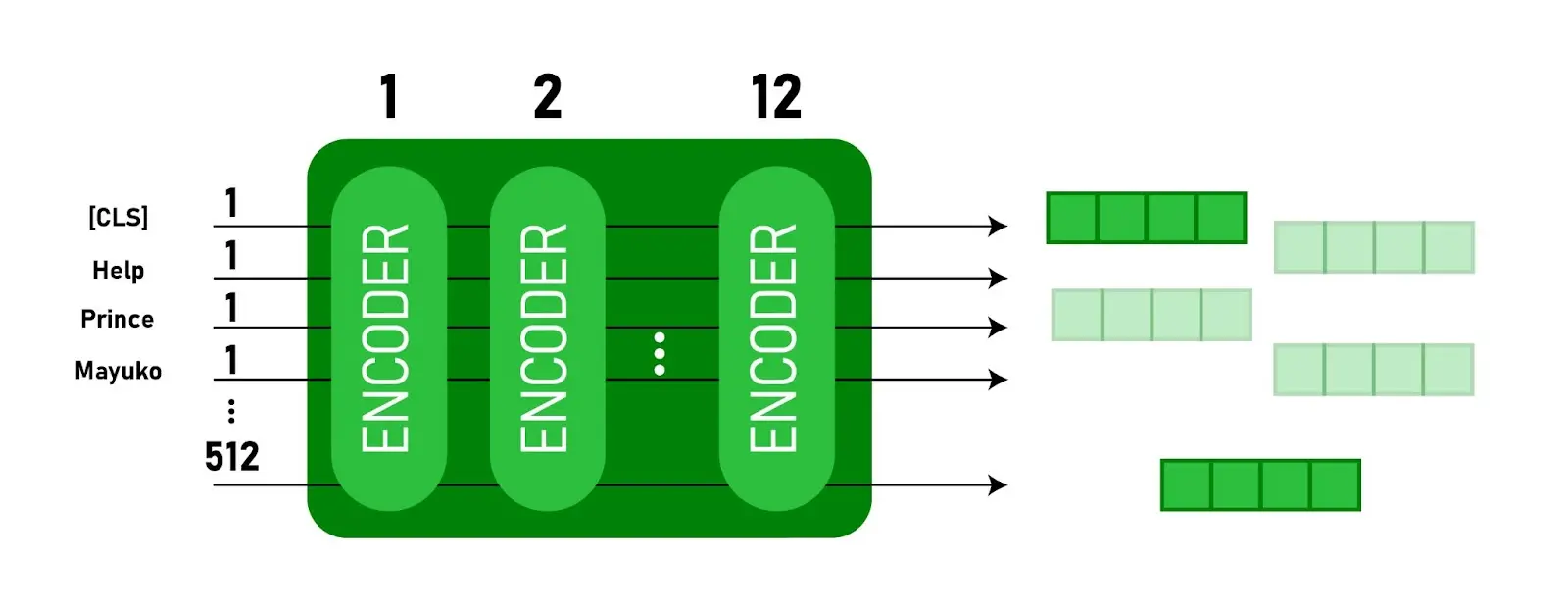
Source
BERT employs a transformer-based architecture, which allows it to capture intricate dependencies and relationships between words in a sentence by simultaneously considering both left and right contexts. Unlike traditional models that train on specific tasks, BERT is pre-trained on a large corpus of text data unsupervised, enabling it to learn general language representations.
These pre-trained representations can then be fine-tuned on downstream NLP tasks such as text classification, named entity recognition, and question answering. BERT has achieved remarkable success across various NLP benchmarks, owing to its ability to capture contextual information and transfer knowledge effectively.
# Loads CSV file
df_bert = pd.read_csv(f'{dir}/fake_news_english.csv')
The following code splits the data into training and test sets using the train_test_split function from scikit-learn.
# Splits data into features and target
X = df_bert['text']
y = df_bert['labels']

# Splits data into training and test sets
X_train, X_test, y_train, y_test = train_test_split(X, y, test_size=0.2, random_state=42)
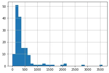
Use the following list comprehension to calculate the sequence length of each text in the X_train dataset by splitting each text into words and calculating the number of words in each text.
# Plots a histogram of the sequence length of the available text
seq_len = [len(i.split()) for i in X_train]

pd.Series(seq_len).hist(bins= 30);
With a clear understanding of the dataset, you can now load your pre-trained BERT model and fine-tune it on your dataset.
Model Training
The code below demonstrates loading a pre-trained BERT model, encoding and preparing the data, defining an optimizer, training the model, and tracking the loss and accuracy metrics during the training process.
import torch
from transformers import BertTokenizer, BertForSequenceClassification
from torch.utils.data import TensorDataset, DataLoader

# Detect if we have a GPU available and set the device accordingly
device = torch.device("cuda" if torch.cuda.is_available() else "cpu")

# Loads the BERT tokenizer
tokenizer = BertTokenizer.from_pretrained('bert-base-uncased', do_lower_case=True)

# Encodes the training and testing set
train_encodings = tokenizer(list(X_train), truncation=True, padding=True, max_length=128)
test_encodings = tokenizer(list(X_test), truncation=True, padding=True, max_length=128)

# Converts the encoded data into PyTorch tensors and move them to the GPU if available
train_inputs = torch.tensor(train_encodings['input_ids']).to(device)
...
The loop iterates over the batches of data, performs forward and backward passes, computes gradients, updates the model’s weights, and calculates the loss and accuracy metrics.
# Trains the model
model.train()
for epoch in range(10):
    running_loss = 0.0
    correct = 0
    total = 0

    for step, batch in enumerate(train_loader):
        ...
        # Updates the weights
        optimizer.step()

        # Accumulates the running loss
        running_loss += loss.item()

        # Predicts labels and calculates the number of correct predictions
        _, predicted = torch.max(outputs.logits, dim=1)
        total += labels.size(0)
        correct += (predicted == labels).sum().item()

    # Calculate accuracy and loss on the entire training set
    accuracy = correct / total
    average_loss = running_loss / len(train_loader)

    # If the current epoch's accuracy is best so far, save the model to disk
    if accuracy > best_accuracy:
        best_accuracy = accuracy
        # torch.save(model.state_dict(), 'best_model.pt')
        torch.save(model, f'{dir}/best_model.pt')

    print(f"Epoch {epoch+1}/{10} - Training Loss: {average_loss:.4f} - Training Accuracy: {accuracy:.4f}")
Output (DO NOT COPY):

Some weights of the model checkpoint at bert-base-uncased were not used when initializing BertForSequenceClassification: ['cls.predictions.transform.dense.weight', 'cls.predictions.transform.dense.bias', 'cls.predictions.transform.LayerNorm.bias', 'cls.seq_relationship.weight', 'cls.predictions.transform.LayerNorm.weight', 'cls.seq_relationship.bias', 'cls.predictions.decoder.weight', 'cls.predictions.bias']
- This IS expected if you are initializing BertForSequenceClassification from the checkpoint of a model trained on another task or with another architecture (e.g. initializing a BertForSequenceClassification model from a BertForPreTraining model).
- This IS NOT expected if you are initializing BertForSequenceClassification from the checkpoint of a model that you expect to be exactly identical (initializing a BertForSequenceClassification model from a BertForSequenceClassification model).
Some weights of BertForSequenceClassification were not initialized from the model checkpoint at bert-base-uncased and are newly initialized: ['classifier.bias', 'classifier.weight']
You should probably TRAIN this model on a down-stream task to be able to use it for predictions and inference.
Epoch 1/10 - Training Loss: 0.3591 - Training Accuracy: 0.8986
Epoch 2/10 - Training Loss: 0.2849 - Training Accuracy: 0.9189
Epoch 3/10 - Training Loss: 0.2271 - Training Accuracy: 0.9257
Epoch 4/10 - Training Loss: 0.1270 - Training Accuracy: 0.9662
Epoch 5/10 - Training Loss: 0.0597 - Training Accuracy: 0.9865
Epoch 6/10 - Training Loss: 0.0367 - Training Accuracy: 0.9932
Epoch 7/10 - Training Loss: 0.0205 - Training Accuracy: 1.0000
Epoch 8/10 - Training Loss: 0.0141 - Training Accuracy: 1.0000
Epoch 9/10 - Training Loss: 0.0127 - Training Accuracy: 1.0000
Epoch 10/10 - Training Loss: 0.0094 - Training Accuracy: 1.0000
Model Evaluation Steps After training a machine learning model, it is crucial to evaluate its performance to assess how well it generalizes to new, unseen data. Model evaluation allows you to measure various metrics that provide insights into the model’s effectiveness. In the following steps, you will evaluate the performance of the trained model using the test set and compute relevant metrics to assess its accuracy and loss.
Here are the steps for this section:
Set the model to evaluation mode: This step ensures that the model is set to evaluation mode, which turns off the computation of gradients and improves inference performance.
Initialize variables to gather the total output: These variables will accumulate the evaluation accuracy, loss, and number of evaluation steps.
Evaluate the data for one epoch: This loop iterates over the batches in the test loader and performs the evaluation steps.
Unpack the batch from the test loader and move tensors to the GPU (if available): This step unpacks the input batch from the test loader and moves the tensors to the GPU if available.
Use torch.no_grad() to turn off gradient computation:
By using the torch.no_grad() context manager, the forward pass is performed without constructing the compute graph, as gradients are unnecessary during evaluation.
Perform a forward pass to calculate logits: The forward pass is executed to obtain the predicted logits from the model for the given input batch.
Retrieve the loss and logits: The loss and logits are obtained from the model’s output.
Accumulate the validation loss: The loss for the current batch is added to the total evaluation loss.
Calculate the accuracy for the batch and accumulate it: The predicted labels are compared to the true labels, and the number of correct predictions is accumulated.
Report the final accuracy for the evaluation: The average accuracy is calculated by dividing the total evaluation accuracy by the total number of samples in the test dataset, providing the overall accuracy on the test set.
Calculate the average loss over all batches: The average test loss is calculated by dividing the total evaluation loss by the number of batches in the test loader.
Print the accuracy on the test set and the test loss: This summarizes the model’s performance on the test set, indicating the accuracy and loss metrics.
# Sets the model to evaluation mode
model.eval()

# Variables to gather full output
total_eval_accuracy = 0
total_eval_loss = 0
nb_eval_steps = 0

# Evaluate data for one epoch
for batch in test_loader:
    # Unpack this training batch from our dataloader and move tensors to GPU if available
    input_ids, attention_mask, labels = [b.to(device) for b in batch]

    # Tells PyTorch not to bother with constructing the compute graph during
    # the forward pass, since this is only needed for backprop (training)
    with torch.no_grad():
        # Forward pass, calculate logit predictions.
        outputs = model(input_ids, attention_mask=attention_mask, labels=labels)

    # Get the loss and logits
    loss = outputs.loss
    logits = outputs.logits

    # Accumulate the validation loss
    total_eval_loss += loss.item()

    # Calculate the accuracy for this batch of test sentences, and accumulate it over all batches
    _, predictions = torch.max(logits, dim=1)
    total_eval_accuracy += (predictions == labels).sum().item()

# Report the final accuracy for this validation run
avg_val_accuracy = total_eval_accuracy / len(test_loader.dataset)
print("Accuracy on the test set: {0:.2f}".format(avg_val_accuracy))

# Calculate the average loss over all of the batches
avg_val_loss = total_eval_loss / len(test_loader)
print("Test Loss: {0:.2f}".format(avg_val_loss))
Output (DO NOT COPY):
Accuracy on the test set: 0.95
Test Loss: 0.23
The accuracy on the test set is 95%, indicating how well the model performs on unseen data. The test loss is 0.23, representing the average loss of the model’s predictions compared to the true labels in the test set.
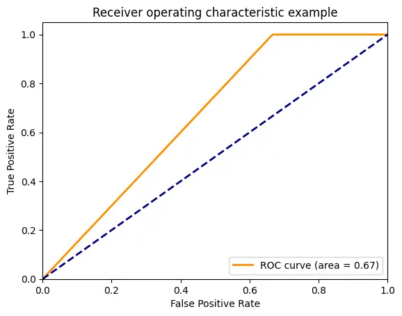
Creating a ROC curve This is similar to evaluating the model in the previous code, although here you’ll create a Reciever Operating Characteristic (ROC) curve.
A ROC (Receiver Operating Characteristic) curve is a graphical representation of the performance of a binary classification model. It plots the true positive rate (sensitivity) against the false positive rate (1 - specificity) for different classification thresholds.
The ROC curve assesses the model’s ability to discriminate between classes and determine an optimal threshold. It provides a visual tool to evaluate the trade-off between the true and false positive rates and helps select the appropriate threshold for a specific classification task.
Here are the steps you’ll follow with the code below:
Set the model to evaluation mode: Prepare the model for evaluation by disabling gradient computation and batch normalization layers.
Create empty lists to store the true and predicted labels: Initialize lists to hold ground truth labels and model predictions.
Iterate over the test data and generate predictions using the model: Loop through the test data batches and use the trained model to generate predictions for each batch.
Convert the predicted logits to a numpy array and extract the predicted labels: Convert the predicted logits (output probabilities) to a numpy array and extract the predicted labels by selecting the class with the highest probability.
Extend the true labels and predicted labels lists with the corresponding values from the current batch: Add the true labels and predicted labels from the current batch to the respective lists.
Compute the ROC curve: Calculate the false positive rate (fpr), true positive rate (tpr), and thresholds for the ROC curve using the true and predicted labels.
Calculate the area under the ROC curve (roc_auc): Measure the model’s overall performance by calculating the area under the ROC curve, which indicates the model’s ability to distinguish between classes.
Plot the ROC curve: Visualize the ROC curve using Matplotlib, with the false positive rate on the x-axis and the true positive rate on the y-axis. Include a label indicating the area under the curve.
Set the axis limits, labels, and titles for the plot: Specify the range and labels for the plot’s x-axis, y-axis, and title.
Display the plot showing the ROC curve: Shows the plot containing the ROC curve to visualize the model’s performance.
# Set the model to evaluation mode
model.eval()

# Lists to store actual and predicted values
true_labels = []
pred_labels = []

# Iterate over the test data and generate predictions
for batch in test_loader:
    input_ids, attention_mask, labels = [b.to(device) for b in batch]

    with torch.no_grad():
        outputs = model(input_ids, attention_mask=attention_mask)

    logits = outputs.logits
    logits = logits.detach().cpu().numpy()

    # Get the predictions and the true labels
    predictions = np.argmax(logits, axis=1)
    true_labels.extend(labels.tolist())
    pred_labels.extend(predictions.tolist())

# Compute ROC curve
fpr, tpr, _ = roc_curve(true_labels, pred_labels)
roc_auc = auc(fpr, tpr)

# Plot ROC curve
plt.figure()
lw = 2  # Line width
plt.plot(fpr, tpr, color='darkorange', lw=lw, label='ROC curve (area = %0.2f)' % roc_auc)
plt.plot([0, 1], [0, 1], color='navy', lw=lw, linestyle='--')
plt.xlim([0.0, 1.0])
plt.ylim([0.0, 1.05])
plt.xlabel('False Positive Rate')
plt.ylabel('True Positive Rate')
plt.title('Receiver operating characteristic example')
plt.legend(loc="lower right")
plt.show()
Testing the Model on Random Article Samples Randomly select “n” number of samples from your DataFrame: Create a new DataFrame test_df containing a random subset of 100 rows from df_bert.
Define the function predict_articles: Define a function that takes test_df, model, and tokenizer as inputs to predict whether each news article in the DataFrame is fake or real using a trained BERT model.
Set the model to evaluation mode: Ensure that the model is in evaluation mode by turning off gradient computation and batch normalization layers.
Iterate over each row in the DataFrame: Loop through each row in the test_df DataFrame.
Extract the article text and true label: Retrieve the article text and true label from the current row.
Encode the article text using the BERT tokenizer: Convert it into tokenized input suitable for the BERT model by encoding it with the tokenizer. Apply truncation, padding, and return attention masks for proper input formatting.
Move tensors to the same device as the model: Transfer the input tensors (input IDs and attention mask) to the same device (CPU or GPU).
Compute model output: Use the model to compute the output logits (raw predictions) by passing the input tensors through the model.
Get the predicted class: Determine the predicted class by selecting the class with the highest probability from the output logits.
Map the predicted class to a label name: Convert the predicted class (0 or 1) to the corresponding label name (“real” or “fake”).
Print the true and predicted labels for the article: Display the true and predicted labels for the current article.
Call the predict_articles function with the test dataframe, model, and tokenizer: Invoke the predict_articles function, passing in the test_df, model, and tokenizer as arguments to predict and print the labels for the articles in the test_df.
randomly creates samples from df_bert
test_df = df_bert.sample(n = 100, random_state = 42)


Define the predict_articles function:

def predict_articles(test_df: pd.DataFrame, model: BertForSequenceClassification, tokenizer: BertTokenizer):
    """
    Predicts whether each news article in a DataFrame is fake or real using a trained BERT model.

    Args:
        test_df (pd.DataFrame): The DataFrame containing the articles.
        model (BertForSequenceClassification): The trained BERT model.
        tokenizer (BertTokenizer): The BERT tokenizer.
    """

    # Ensure the model is in evaluation mode
    model.eval()

    # Iterate over each row in the DataFrame
    for i, row in test_df.iterrows():
        # Extract the article and true label
        article = row['text']
        true_label = 'Real' if row['labels'] == 0 else 'Fake'

        # Encode the article text
        encoded_text = tokenizer.encode_plus(
            article,
            add_special_tokens=True,
            max_length=512,
            padding='max_length',
            truncation=True, # truncates the text to the specified max_length
            return_attention_mask=True,
            return_tensors='pt'
        )

        # Move tensors to the same device as the model
        input_ids = encoded_text['input_ids'].to(device)
        attention_mask = encoded_text['attention_mask'].to(device)

        # Compute model output
        with torch.no_grad():
            outputs = model(input_ids, attention_mask=attention_mask)

        # Get the predicted class
        predicted_class = torch.argmax(outputs.logits, dim=1).item()

        # Map the predicted class to a label name
        predicted_label = 'Real' if predicted_class == 0 else 'Fake'

        # Print the true and predicted labels for the article
        print(f"Article {i+1}:")
        print(f"  True label:     {true_label}")
        print(f"  Predicted label: {predicted_label}\n")
        print("=====================================")

# Call the function with your test dataframe, model, and tokenizer
predict_articles(test_df, model, tokenizer)
Output (DO NOT COPY):
Article 114:
  True label:     Fake
  Predicted label: Fake

=====================================
Article 165:
  True label:     Fake
  Predicted label: Fake

=====================================
Article 170:
  True label:     Real
  Predicted label: Fake

=====================================
Article 102:
  True label:     Fake
  Predicted label: Fake

=====================================
Article 101:
  True label:     Fake
  Predicted label: Fake

=====================================
Article 16:
  True label:     Fake
  Predicted label: Fake

=====================================
Article 178:
  True label:     Real
  Predicted label: Fake

=====================================
Article 36:
  True label:     Fake
  Predicted label: Fake

=====================================
Article 120:
  True label:     Fake
  Predicted label: Fake
Conclusion
In this PyTorch walkthrough tutorial on creating a fake news classification model, you have learned how to:
Preprocess the text data: You tokenized the text, converted it into numerical representations (input IDs), and create attention masks to handle variable-length sequences.
Load and prepare the data: You loaded the fake news dataset, split it into training and testing sets, created data loaders for efficient batch processing, and handle class imbalance using techniques like oversampling or undersampling.
Build a fine-tuned BERT model with Pytorch: You loaded a pre-trained BERT model, modify it for sequence classification, and adapt it to your specific task of fake news detection.
Train the model with Pytorch: You learned how to define the training loop, perform forward and backward passes, update model parameters using gradient descent, and monitor the training progress with metrics like loss and accuracy.
Evaluate the model: You evaluated the trained model on a separate test set, calculated metrics such as accuracy and loss, and interpreted the results to assess the model’s performance.
Throughout this tutorial, you gained insights into the PyTorch framework, its powerful capabilities for natural language processing (NLP), and its application in creating a fake news classification model.
By following the step-by-step instructions and understanding the underlying concepts, you are now equipped with the knowledge and skills to apply PyTorch to some NLP tasks and build your own classification models. Remember, keep experimenting, exploring, and refining your ML skills.
Happy coding!