
This article was published when data science tooling like Dask and R was a primary focus for Saturn Cloud. Today, Saturn Cloud is the enterprise AI platform for any GPU infrastructure.
As data scientists, we often encounter scenarios where we need to analyze the trends and patterns in our data. One common task is calculating slopes, which can provide valuable insights into the rate of change of a variable over time or across different dimensions. In this blog post, we will explore how to calculate slopes using the powerful NumPy and SciPy libraries, and discuss their applications in data analysis.
Table of Contents
- Introduction
- Understanding Slopes
- Calculating Slopes with NumPy
- Calculating Slopes with SciPy
- Applications of Slope Calculation
- 5.1 Trend Analysis
- 5.2 Forecasting
- 5.3 Anomaly Detection
- Pros and Cons of Slope Calculation with NumPy and SciPy
- Error Handling
- Conclusion
Understanding Slopes
Before we dive into the implementation details, let’s briefly review what slopes represent in the context of data analysis. In simple terms, a slope measures the steepness of a line or curve. It quantifies the rate of change between two points on a graph. Slopes are commonly used to analyze trends, identify patterns, and make predictions based on historical data.
Calculating Slopes with NumPy
NumPy is a fundamental library for scientific computing in Python, providing powerful array manipulation capabilities. It offers a range of mathematical functions, including functions for calculating slopes.
To calculate slopes using NumPy, we can leverage the numpy.gradient() function. This function computes the gradient of an N-dimensional array. In the context of calculating slopes, we are primarily interested in the gradient along a specific axis.
Let’s consider a simple example where we have a one-dimensional array representing a time series of data points. We want to calculate the slope for each point in the time series. Here’s how we can achieve this using NumPy:
import numpy as np

# Generate sample data
time_series = np.array([1, 2, 4, 7, 11, 16, 22])

# Calculate slopes
slopes = np.gradient(time_series)

print(slopes)
Output
[1. 1.5 2.5 3.5 4.5 5.5 6. ]
In this example, we first generate a sample one-dimensional array called time_series. We then use the numpy.gradient() function to calculate the slopes for each point in the time_series array. The resulting slopes are stored in the slopes variable and printed to the console.
Each value in the resulting array represents the slope or the rate of change at the corresponding point in the time_series. For example, the first value of 1.0 means that between the first and second points in the time_series, the rate of change is 1.0. Similarly, the second value of 1.5 means that between the second and third points, the rate of change is 1.5, and so on.
The resulting slopes represent the rate of change at each point in the time series. Now, let’s visualize these slopes:
import matplotlib.pyplot as plt

# Plot the time series
plt.plot(time_series, marker='o', label='Time Series')

# Add labels and legend
plt.xlabel('Index')
plt.ylabel('Value')
plt.title('Time Series and Slopes')
plt.legend()

# Show the plot
plt.show()
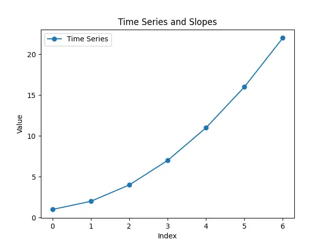
This graph overlays the original time series with a dashed line representing the calculated slopes. Each point on the dashed line corresponds to the slope at the respective index in the time series.
By visually inspecting the graph, we can observe how the slopes capture the varying rates of change in the time series data.
Calculating Slopes with SciPy
SciPy is a powerful library for scientific and technical computing in Python. It builds upon NumPy and provides additional functionality, including advanced mathematical algorithms. SciPy offers a dedicated module called scipy.stats that provides various statistical functions, including a function for calculating slopes.
To calculate slopes using SciPy, we can utilize the scipy.stats.linregress() function. This function performs a linear regression on two sets of measurements and returns several statistical parameters, including the slope of the regression line.
Let’s take a look at an example that demonstrates how to calculate slopes using SciPy:
import numpy as np
from scipy import stats

# Generate sample data
x = np.array([0, 1, 2, 3, 4, 5, 6])
y = np.array([1, 2, 4, 7, 11, 16, 22])

# Calculate slope using linear regression
slope, intercept, r_value, p_value, std_err = stats.linregress(x, y)

print(slope)
Output:
3.5
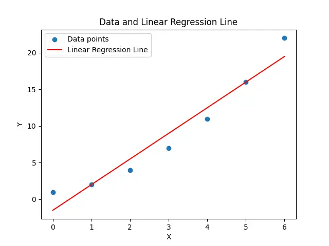
In this example, we define two arrays x and y representing the x and y coordinates of a set of data points. We then use the scipy.stats.linregress() function to calculate the slope of the linear regression line fitting the data points. The resulting slope is stored in the slope variable and printed to the console.
Applications of Slope Calculation
Now that we have explored how to calculate slopes using NumPy and SciPy, let’s discuss some practical applications of slope calculation in data analysis:
Trend Analysis
Slope calculation is commonly used to analyze trends in time series data. By calculating the slopes over a specific period, we can determine whether the data is increasing, decreasing, or remaining constant. This information is crucial for making informed decisions and predictions based on the observed trends.
Forecasting
By analyzing the slopes of historical data, we can make predictions about future trends and patterns. For example, if the slopes indicate a steady increase, we can forecast future values to be higher. Similarly, if the slopes indicate a decline, we can anticipate a downward trend.
Anomaly Detection
Slope calculation can also be useful for detecting anomalies or outliers in data. Unusual slopes that deviate significantly from the expected patterns can indicate the presence of abnormal data points. Identifying such anomalies is crucial for ensuring data quality and making informed decisions based on reliable information.
Pros and Cons of Slope Calculation with NumPy and SciPy
Pros
Efficiency and Performance: Both NumPy and SciPy are highly optimized libraries for numerical and scientific computing in Python. They provide efficient implementations for mathematical operations, making slope calculations fast and reliable, even for large datasets.
Versatility: The NumPy and SciPy libraries are versatile and can handle a wide range of mathematical operations beyond slope calculations. This makes them suitable for a variety of data analysis tasks, providing a comprehensive toolkit for data scientists.
Community Support: NumPy and SciPy have large and active communities. This means that users can find ample documentation, tutorials, and community forums where they can seek help, share insights, and stay updated on best practices in numerical computing.
Integration with Other Libraries: NumPy and SciPy integrate seamlessly with other popular Python libraries used in data science, such as Pandas, Matplotlib, and scikit-learn. This allows data scientists to build end-to-end data analysis pipelines efficiently.
Cons
Learning Curve: For beginners, the syntax and functionality of NumPy and SciPy might have a steeper learning curve compared to simpler libraries. Understanding the full capabilities of these libraries may take some time, especially for those new to scientific computing.
Resource Consumption: NumPy and SciPy may consume more memory, especially when dealing with large datasets. Careful consideration of memory management is required to avoid performance issues on systems with limited resources.
Not Always Necessary: For simpler tasks or smaller datasets, using these powerful libraries might be overkill. In such cases, simpler solutions or libraries might be more appropriate and easier to implement.
Error Handling
Input Validation: Ensure that input data provided to functions like
numpy.gradient()orscipy.stats.linregress()is valid and appropriate for the intended calculations. Invalid inputs may lead to unexpected errors or inaccurate results.Handling NaN Values: Real-world datasets often contain missing or invalid values. Implement robust strategies to handle NaN (Not a Number) values that may arise during slope calculations, preventing them from propagating and affecting downstream analyses.
Model Assumptions: Understand the assumptions underlying the methods used (e.g., linear regression assumptions in
scipy.stats.linregress()). Check for violations of these assumptions, and handle cases where the assumptions may not be met appropriately.Documentation and Error Messages: Clearly document the code and use descriptive variable names. Additionally, incorporate error-checking mechanisms and provide informative error messages to aid in debugging and understanding potential issues during code execution.
Conclusion
Calculating slopes is a fundamental task in data analysis, providing valuable insights into trends, patterns, and relationships in data. In this blog post, we explored how to calculate slopes using two powerful Python libraries, NumPy and SciPy. We discussed the implementation details and showcased practical applications of slope calculation in various data analysis scenarios. By leveraging these techniques, data scientists can gain deeper insights into their data and make more informed decisions.