What Is Sklearn PCA Explained Variance and Explained Variance Ratio Difference?

If you’re a data scientist or software engineer, you’ve probably heard of PCA, or Principal Component Analysis. PCA is a widely used technique in data science and machine learning for dimensionality reduction, which is the process of reducing the number of features in a dataset while preserving as much of the original information as possible.

One important aspect of PCA is the concept of explained variance, which measures how much of the total variance in the original dataset is explained by each principal component. In this blog post, we’ll explain the difference between explained variance and explained variance ratio in Sklearn PCA, and how to interpret them.

Table of Contents

1. Introduction
2. What is Sklearn PCA?
3. Explained Variance in Sklearn PCA
   • Code Example
4. Explained Variance Ratio in Sklearn PCA
   • Code Example
   • Variance Ratio Plot
5. Interpreting Explained Variance and Explained Variance Ratio
6. Pros and Cons of Sklearn PCA
   • Pros
   • Cons
7. Error Handling in Sklearn PCA
8. Conclusion

What is Sklearn PCA?

Sklearn PCA is a Python library that provides a simple and efficient implementation of PCA for dimensionality reduction. Sklearn PCA can be used for a variety of tasks, such as data compression, feature extraction, and data visualization.

The Sklearn PCA algorithm works by finding the principal components of a dataset, which are the directions in which the data varies the most. These principal components are ordered by the amount of variance they explain in the original dataset, with the first principal component explaining the most variance, the second explaining the second most variance, and so on.

Explained Variance in Sklearn PCA

Explained variance is a measure of how much of the total variance in the original dataset is explained by each principal component. The explained variance of a principal component is equal to the eigenvalue associated with that component.

In Sklearn PCA, the explained variance of each principal component can be accessed through the explained_variance_ attribute. For example, if pca is a Sklearn PCA object, pca.explained_variance_[i] gives the explained variance of the i-th principal component.

The total explained variance of a set of principal components is simply the sum of the explained variance of those components. In Sklearn PCA, the total explained variance of the first k principal components can be accessed through the explained_variance_ attribute as follows:

pca.explained_variance_[:k].sum()

Example:

# Import necessary libraries
from sklearn.decomposition import PCA
from sklearn.datasets import make_classification

# Generate a synthetic dataset
X, y = make_classification(n_samples=1000, n_features=20, n_informative=10, n_redundant=5, random_state=42)

# Apply PCA
pca = PCA()
X_pca = pca.fit_transform(X)

# Explained variance
explained_variance = pca.explained_variance_
total_explained_variance = explained_variance.sum()

# Print results
print(f"Explained Variance:\n{explained_variance}")
print(f"Total Explained Variance: {total_explained_variance:.4f}")

Output:

Explained Variance:
[2.72241687e+01 2.06879375e+01 1.88626814e+01 1.13944715e+01
 7.12127027e+00 5.51297019e+00 4.06031069e+00 3.90237182e+00
 2.65652213e+00 1.92169023e+00 1.10493122e+00 1.03809743e+00
 1.00397775e+00 9.39230877e-01 8.67446654e-01 2.62547731e-30
 2.17731849e-30 1.18617768e-30 4.82693715e-31 2.38257402e-31]
Total Explained Variance: 108.2981

Explained Variance Ratio in Sklearn PCA

Explained variance ratio is a measure of the proportion of the total variance in the original dataset that is explained by each principal component. The explained variance ratio of a principal component is equal to the ratio of its eigenvalue to the sum of the eigenvalues of all the principal components.

In Sklearn PCA, the explained variance ratio of each principal component can be accessed through the explained_variance_ratio_ attribute. For example, if pca is a Sklearn PCA object, pca.explained_variance_ratio_[i] gives the explained variance ratio of the i-th principal component.

The total explained variance ratio of a set of principal components is simply the sum of the explained variance ratios of those components. In Sklearn PCA, the total explained variance ratio of the first k principal components can be accessed through the explained_variance_ratio_ attribute as follows:

pca.explained_variance_ratio_[:k].sum()

Example:

# Explained variance ratio
explained_variance_ratio = pca.explained_variance_ratio_
total_explained_variance_ratio = explained_variance_ratio.sum()

# Print results
print(f"\nExplained Variance Ratio:\n{explained_variance_ratio}")
print(f"Total Explained Variance Ratio: {total_explained_variance_ratio:.4f}")

Output:

Explained Variance Ratio:
[2.51381826e-01 1.91027743e-01 1.74173740e-01 1.05213977e-01
 6.57562016e-02 5.09055218e-02 3.74919920e-02 3.60336202e-02
 2.45297254e-02 1.77444536e-02 1.02026854e-02 9.58555726e-03
 9.27050381e-03 8.67264583e-03 8.00980652e-03 2.42430646e-32
 2.01048672e-32 1.09528969e-32 4.45708476e-33 2.20001505e-33]
Total Explained Variance Ratio: 1.0000

# Import necessary libraries
import numpy as np
import matplotlib.pyplot as plt

# Plot explained variance ratio
cumulative_variance_ratio = np.cumsum(explained_variance_ratio)
plt.plot(cumulative_variance_ratio, marker='o')
plt.xlabel('Number of Principal Components')
plt.ylabel('Cumulative Explained Variance Ratio')
plt.title('Cumulative Explained Variance Ratio by Principal Components')
plt.show()

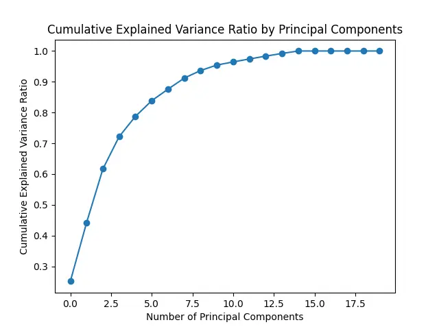
The plot above illustrates the cumulative explained variance ratio by the number of principal components. Each point on the curve represents the cumulative proportion of total variance explained as we incrementally add principal components. This visualization can help in determining the optimal number of principal components to retain, balancing the goal of dimensionality reduction with preserving a sufficient amount of information from the original dataset.

Interpreting Explained Variance and Explained Variance Ratio

Explained variance and explained variance ratio are both measures of how much of the total variance in the original dataset is explained by each principal component. However, they differ in their interpretation.

Explained variance measures the absolute amount of variance that is explained by each principal component. This is useful when you want to know how many principal components you need to retain in order to capture a certain percentage of the total variance in the original dataset.

Explained variance ratio measures the relative amount of variance that is explained by each principal component. This is useful when you want to know how much information each principal component contributes to the overall structure of the data.

For example, suppose you have a dataset with 100 features, and you perform Sklearn PCA with 10 principal components. The total explained variance of the first 10 principal components is 80%, which means that these 10 principal components capture 80% of the total variance in the original dataset.

Suppose further that the explained variance ratio of the first principal component is 50%. This means that the first principal component explains 50% of the total variance in the original dataset, and is therefore the most important principal component. The second principal component might have an explained variance ratio of 20%, which means that it explains 20% of the total variance in the original dataset, and is therefore less important than the first principal component.

Pros and Cons of Sklearn PCA

Pros

1. Dimensionality Reduction: Sklearn PCA is a powerful tool for reducing the dimensionality of a dataset by capturing the most significant variations in the data through principal components.
2. Computationally Efficient: Sklearn PCA is implemented in a highly efficient manner, making it suitable for large datasets. It uses techniques such as singular value decomposition (SVD) for numerical stability.
3. Data Compression: PCA allows for effective data compression, especially in scenarios where the original dataset has a large number of features, by retaining a smaller set of principal components.
4. Interpretability: The principal components obtained through PCA are orthogonal and represent uncorrelated features, which can enhance the interpretability of the transformed data.
5. Noise Reduction: PCA can help in reducing noise and capturing the underlying patterns in the data, leading to a more robust representation.

Cons

1. Loss of Interpretability: While PCA enhances interpretability in some cases, it may also lead to a loss of interpretability as the transformed features are linear combinations of the original features.
2. Assumption of Linearity: PCA assumes that the underlying structure in the data is linear. If the data has a nonlinear structure, PCA may not perform optimally.
3. Sensitive to Outliers: PCA is sensitive to outliers in the dataset, and outliers can disproportionately influence the principal components.
4. Calculation of Eigenvectors and Eigenvalues: The computation of eigenvectors and eigenvalues, which are fundamental to PCA, can be computationally expensive for very large datasets.

Error Handling in Sklearn PCA:

When using Sklearn PCA, it’s essential to consider potential errors and handle them appropriately. Here are some common errors and suggestions for handling them:

1. Insufficient Data: If the dataset is too small, PCA may not provide reliable results. Ensure that your dataset has enough samples to capture meaningful variations.
2. Inconsistent Data Types: PCA requires numerical data. Ensure that all features in your dataset are numerical, and consider preprocessing steps for categorical data.
3. Scaling Issues: PCA is sensitive to the scale of features. Standardize or normalize the features before applying PCA to ensure that all features contribute equally.
4. Zero or Low Variance Features: Features with zero or very low variance do not contribute much information. Identify and remove such features before applying PCA.
5. Out-of-Memory Errors: For large datasets, memory issues may arise. Consider using incremental PCA or applying PCA on a representative subset of the data.

Conclusion

Sklearn PCA is a powerful technique for dimensionality reduction, and explained variance and explained variance ratio are important measures for interpreting the results of Sklearn PCA. In this blog post, we’ve explained the difference between explained variance and explained variance ratio in Sklearn PCA, and how to interpret them.

Remember that while explained variance measures the absolute amount of variance explained by each principal component, explained variance ratio measures the relative amount of variance explained by each principal component. Understanding the difference between these two measures is crucial for interpreting the results of Sklearn PCA and making informed decisions about the number of principal components to retain.

SHARE:

About Saturn Cloud

Saturn Cloud is your all-in-one solution for data science & ML development, deployment, and data pipelines in the cloud. Spin up a notebook with 4TB of RAM, add a GPU, connect to a distributed cluster of workers, and more. Request a demo today to learn more.