Multi-class logistic regression with TensorFlow 2.0: A comprehensive guide

As data scientists and software engineers, we know that building accurate machine learning models is essential for any project that involves data analysis. One of the most popular techniques for classification problems is logistic regression. In this post, we’ll explore the concept of multi-class logistic regression and how to implement it using TensorFlow 2.0 with the common IRIS Dataset.

Table of Contents

1. What is multi-class logistic regression?
2. How does multi-class logistic regression work?
3. Implementing multi-class logistic regression with TensorFlow 2.0
4. Common Errors and How to Handle Them
5. Conclusion

What is multi-class logistic regression?

Logistic regression is a statistical method that allows you to analyze the relationship between a dependent variable and one or more independent variables. In binary logistic regression, the dependent variable is binary, which means it has two possible values (0 or 1). On the other hand, in multi-class logistic regression, the dependent variable can have more than two possible values.

Multi-class logistic regression is also known as softmax regression. It is a generalization of binary logistic regression that allows you to classify data into more than two categories. In this method, you calculate the probability of each category and then select the category with the highest probability as the predicted class.

How does multi-class logistic regression work?

In multi-class logistic regression, the goal is to find a set of weights and biases that best predicts the probability of each class. To achieve this, we use a softmax function that converts the outputs of the model into probabilities.

The softmax function takes a vector of real numbers as input and returns a probability distribution that sums to one. The formula for the softmax function is as follows:

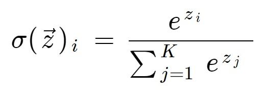
where zi is the i-th element of the input vector and K is the number of classes.

The output of the softmax function is a vector of probabilities that represents the likelihood of each class. The predicted class is the one with the highest probability.

Implementing multi-class logistic regression with TensorFlow 2.0

Now that we understand what multi-class logistic regression is and how it works, let’s see how we can implement it using TensorFlow 2.0.

Loading the data

For this example, we’ll use the famous Iris dataset, which contains information about the petal and sepal length and width of three species of iris flowers. The goal is to predict the species of the flower based on its measurements.

First, we’ll load the dataset and split it into training and test sets:

import tensorflow as tf
from sklearn.datasets import load_iris
from sklearn.model_selection import train_test_split

# Load the Iris dataset
iris = load_iris()

# Split the dataset into training and test sets
X_train, X_test, y_train, y_test = train_test_split(
    iris.data, iris.target, test_size=0.2, random_state=42)

Preprocessing the data

Before we can train our model, we need to preprocess the data. In this case, we’ll normalize the features to have zero mean and unit variance:

# Normalize the features
mean = X_train.mean(axis=0)
std = X_train.std(axis=0)
X_train = (X_train - mean) / std
X_test = (X_test - mean) / std

Defining the model

Next, we’ll define our model using the Keras API, which is integrated into TensorFlow 2.0. We’ll use a sequential model with one hidden layer and a softmax output layer:

# Define the model
model = tf.keras.Sequential([
    tf.keras.layers.Dense(10, activation='relu', input_shape=(4,)),
    tf.keras.layers.Dense(3, activation='softmax')
])

In this model, the first layer is a fully connected layer with 10 hidden units and a ReLU activation function. The second layer is the output layer with three units, one for each class, and a softmax activation function.

Compiling the model

Before we can train the model, we need to compile it. We’ll use the categorical_crossentropy loss function, which is suitable for multi-class classification problems, and the Adam optimizer:

# Compile the model
model.compile(optimizer='adam',
              loss='sparse_categorical_crossentropy',
              metrics=['accuracy'])

Training the model

Now we’re ready to train our model. We’ll use the fit() method to train the model for 50 epochs:

# Train the model
history = model.fit(X_train, y_train, epochs=50, validation_split=0.2)

Evaluating the model

Once the model is trained, we can evaluate its performance on the test set:

# Evaluate the model
loss, accuracy = model.evaluate(X_test, y_test)
print('Test accuracy:', accuracy)

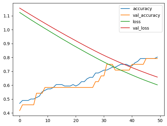
Visualizing the results

Finally, we can visualize the training and validation accuracy and loss using Matplotlib:

import matplotlib.pyplot as plt

# Plot the accuracy and loss
plt.plot(history.history['accuracy'], label='accuracy')
plt.plot(history.history['val_accuracy'], label='val_accuracy')
plt.plot(history.history['loss'], label='loss')
plt.plot(history.history['val_loss'], label='val_loss')
plt.legend()
plt.show()

Common Errors and How to Handle Them

Divergence during Training:

Issue:

When training the model, you observe that the loss diverges, meaning it increases instead of converging to a minimum. This divergence can prevent the model from learning effectively.

Solution:

Experiment with different learning rates. The learning rate determines the size of the steps taken during the optimization process. If the learning rate is too high, it can cause the model to overshoot the minimum, leading to divergence. Conversely, if it’s too low, the model may converge very slowly or get stuck in local minima. Gradually decrease the learning rate if divergence persists. Additionally, consider using adaptive optimizers like Adam, which adjust the learning rates during training.

# Example of using the Adam optimizer
optimizer = tf.keras.optimizers.Adam(learning_rate=0.001)
model.compile(optimizer=optimizer, loss='categorical_crossentropy', metrics=['accuracy'])

Overfitting:

Issue:

Your model performs exceptionally well on the training set but fails to generalize to new, unseen data, performing poorly on the test set. This phenomenon is known as overfitting.

Solution:

Introduce regularization techniques to prevent overfitting. Two common approaches are dropout and L2 regularization. Dropout randomly drops a percentage of neurons during training, preventing the model from relying too heavily on specific neurons. L2 regularization adds a penalty term to the loss function, discouraging the model from assigning excessively large weights to features.

# Example of adding dropout to a model
model = tf.keras.models.Sequential([
    tf.keras.layers.Dense(128, activation='relu', input_shape=(4,)),
    tf.keras.layers.Dropout(0.5),  # Add dropout layer with a dropout rate of 0.5
    tf.keras.layers.Dense(3, activation='softmax')
])

# Example of adding L2 regularization to a layer
model.add(tf.keras.layers.Dense(64, activation='relu', kernel_regularizer=tf.keras.regularizers.l2(0.01)))

Data Mismatch:

Issue:

There’s a mismatch between the distributions of the training and testing datasets, leading to poor model performance on new data.

Solution:

Ensure that the training and testing datasets are representative of the overall data distribution. Carefully curate datasets to include diverse examples of each class. If a significant mismatch exists, performance on the test set may not reflect the model’s true ability to generalize. Additionally, consider data augmentation techniques to artificially increase the diversity of your training data, ensuring the model encounters a wide range of scenarios.

# Example of using data augmentation with Keras
from tensorflow.keras.preprocessing.image import ImageDataGenerator

datagen = ImageDataGenerator(
    rotation_range=40,
    width_shift_range=0.2,
    height_shift_range=0.2,
    shear_range=0.2,
    zoom_range=0.2,
    horizontal_flip=True,
    fill_mode='nearest'
)

# Apply data augmentation to the training set
datagen.fit(X_train)

Conclusion

In this post, we’ve explored the concept of multi-class logistic regression and how to implement it using TensorFlow 2.0. We’ve seen that multi-class logistic regression is a powerful technique for classification problems with more than two categories. We’ve also seen how to load and preprocess data, define and compile a model, and train and evaluate the model. By following these steps, you can build accurate machine learning models for your own classification problems.

SHARE:

About Saturn Cloud

Saturn Cloud is your all-in-one solution for data science & ML development, deployment, and data pipelines in the cloud. Spin up a notebook with 4TB of RAM, add a GPU, connect to a distributed cluster of workers, and more. Request a demo today to learn more.