Integrative analysis of single-cell multiomics data using deep learning

In this tutorial, we have built an autoencoder-based deep learning model for dimensionality reduction and visualization of single-cell CITE-seq data. We demonstrate that the integrative analysis of both transcriptomic and proteomic data achieves superior resolution in distinguishing between various immune cell types.

By Yuan Tian | Monday, August 29, 2022 | Updated: Tuesday, October 03, 2023

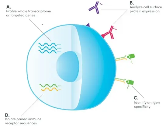
Single-cell RNA sequencing (scRNA-seq) has offered a comprehensive and unbiased approach to profile various type of cells such as immune cells with a single-cell resolution using next‑generation sequencing. More recently, exciting technologies such as cellular indexing of transcriptomes and epitopes by sequencing (CITE-seq) have been developed to extend scRNA-seq by jointly measuring multiple molecular modalities such as proteome and transcriptome from the same cell as illustrated in the figure below. By utilizing antibodies that are conjugated to oligonucleotides, CITE-seq simultaneously generates sequencing-based readouts for surface protein expression along with gene expression.

Since gene and protein expressions convey distinct and complementary information about a cell, CITE-seq offers a unique opportunity to combine both transcriptomic and proteomic data to decipher the biology of individual cells at a considerably higher resolution than using either one alone. This requires computational methods that can effectively integrate single-cell data from both modalities. In this tutorial, we will conduct integrative analysis of CITE-seq data using an unsupervised deep learning method named autoencoder.

In essence:

Single-cell technologies offer considerable promise in dissecting the heterogeneity among individual cells and are being utilized in biomedical studies at an astounding pace.
CITE-seq simultaneously measures gene expression and surface protein at a single-cell level.

Image source: 10x Genomics

# Standard libraries
import time
import pandas as pd
import [numpy](https://saturncloud.io/glossary/numpy) as np
import urllib.request
from pathlib import Path
from urllib.error import HTTPError
from tqdm.notebook import tqdm 
from sklearn import preprocessing

# Pytorch and [Pytorch Lightning](https://saturncloud.io/glossary/pytorch-lightning)
import torch
import torch.nn as nn
import torch.nn.functional as F
import torch.optim as optim
import pytorch_lightning as pl
from torch.utils.data import Dataset, DataLoader, random_split
from pytorch_lightning.callbacks import LearningRateMonitor, ModelCheckpoint

# Visualization and plotting
import umap
import [plotly](https://saturncloud.io/glossary/plotly).express as px

# Tensorboard extension
from torch.utils.tensorboard import SummaryWriter
%load_ext tensorboard

# Path to datasets
DATASET_PATH = Path("data")
if not DATASET_PATH.exists():
    DATASET_PATH.mkdir()
    
# Path to saved models
CHECKPOINT_PATH = Path("saved_models")
if not CHECKPOINT_PATH.exists():
    CHECKPOINT_PATH.mkdir()

# for reproducibility 
pl.seed_everything(42)
torch.backends.cudnn.deterministic = True
torch.backends.cudnn.benchmark = False

# Use [GPU](https://saturncloud.io/glossary/gpu) if available, otherwise use cpu instead 
device = torch.device("cuda:0") if torch.cuda.is_available() else torch.device("cpu")
print("Device:", device)

Data

We will be using the CITE-seq dataset published by Stuart and Butler et al. in 2019. The authors measured the single-cell transcriptomics of 30,672 bone marrow cells together with the expression of 25 proteins. I have already preprocessed the data to generate normalized counts and cell type anonations using Seurat, which is a popular R package for analyzing single-cell genomics data. The script used for preprocessing can be found here. There are three CSV files (RNA, protein, and cell type annotation), which can be downloaded from my github repo using the code below:

# URL for downloading data
data_url = "https://raw.githubusercontent.com/naity/citeseq_autoencoder/master/data/"

# Files to download
data_files = ["rna_scale.csv.gz", "protein_scale.csv.gz", "metadata.csv.gz"]

# Download datafile if necessary
for file_name in data_files:
    file_path = Path(DATASET_PATH/file_name)
    if not file_path.exists():
        file_url = data_url + file_name
        print(f"Downloading {file_url}...")
        try:
            urllib.request.urlretrieve(file_url, file_path)
        except HTTPError as e:
            print("Something went wrong. Please try downloading the file from the Google Drive folder\n", e)

# use [Pandas](https://saturncloud.io/glossary/pandas) to read the data
rna = pd.read_csv(DATASET_PATH/"rna_scale.csv.gz", index_col=0).T
pro = pd.read_csv(DATASET_PATH/"protein_scale.csv.gz", index_col=0).T

ncells = rna.shape[0]
nfeatures_rna = rna.shape[1]
nfeatures_pro = pro.shape[1]

print("Number of cells:", ncells)
print("Number of genes:", nfeatures_rna)
print("Number of proteins:", nfeatures_pro)

Next, gene and protein expression data are concatenated together, where each column is a gene or protein while each row is a cell (each cell has a unique barcode). The dataset contains the expression levels of 2000 genes and 25 proteins for a total of 30672 cells. We will also import the annotations of each cell for visualizaiton purpose later.

# concat rna and pro
assert all(rna.index == pro.index), "RNA and protein data cell barcodes do not match!"
citeseq = pd.concat([rna, pro], axis=1)
print(citeseq.shape)
citeseq.head()

# cell type annotations
metadata = pd.read_csv(DATASET_PATH/"metadata.csv.gz", index_col=0)
metadata.head()

assert all(citeseq.index == pro.index), "CITE-seq data and metadata cell barcodes do not match!"

# separate CD4 and CD8 in l1
metadata["celltype.l1.5"] = metadata["celltype.l1"].values
metadata.loc[metadata["celltype.l2"].str.startswith("CD4"), "celltype.l1.5"] = "CD4 T"
metadata.loc[metadata["celltype.l2"].str.startswith("CD8"), "celltype.l1.5"] = "CD8 T"
metadata.loc[metadata["celltype.l2"]=="Treg", "celltype.l1.5"] = "CD4 T"
metadata.loc[metadata["celltype.l2"]=="MAIT", "celltype.l1.5"] = "MAIT"
metadata.loc[metadata["celltype.l2"]=="gdT", "celltype.l1.5"] = "gdT"

# convert cell type annoations to integers
le = preprocessing.LabelEncoder()
labels = le.fit_transform(metadata["celltype.l1.5"])

Pytorch datasets and dataloaders

class TabularDataset(Dataset):
    """Custome dataset for tabular data"""
    def __init__(self, df: pd.DataFrame, labels: np.ndarray):
        self.data = torch.tensor(df.to_numpy(), dtype=torch.float)
        self.labels = torch.tensor(labels, dtype=torch.float)

    def __len__(self):
        return len(self.data)

    def __getitem__(self, idx):
        x = self.data[idx]
        y = self.labels[idx]
        return x, y

dataset = TabularDataset(citeseq, labels)

# train, validation, and test split
train_size = int(ncells*0.7)
val_size = int(ncells*0.15)
train_ds, val_ds, test_ds = random_split(dataset, [train_size, val_size, ncells-train_size-val_size],
                                         generator=torch.Generator().manual_seed(0))

print("Number of cells for training:", len(train_ds))
print("Number of cells for validation:", len(val_ds))
print("Number of cells for test:", len(test_ds))

# batch size
bs = 256

train_dl = DataLoader(train_ds, batch_size=bs, shuffle=True, drop_last=True, pin_memory=True)
val_dl = DataLoader(val_ds, batch_size=bs, shuffle=False, drop_last=False)
test_dl = DataLoader(test_ds, batch_size=bs, shuffle=False, drop_last=False)

Let’s look at one example of the dataset:

x, y = train_dl.dataset[0]
print("Input data:", x)
print("Label:     ", y)

Use autoencoders for single-cell analysis

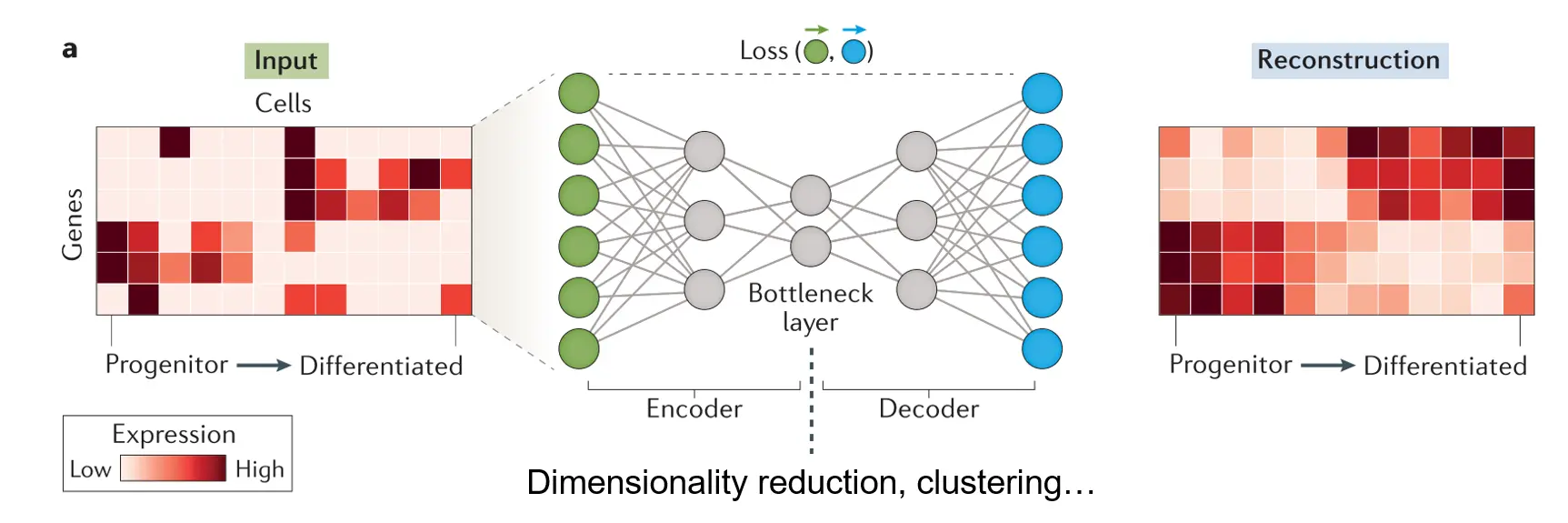
Autoencoder is a type of unsupervised deep learning model or neural network that consists of three major components: an encoder, a bottleneck, and a decoder as shown in the figure below. The encoder compresses the input, and the bottleneck layer stores the compressed representation of the input. In contrast, the decoder tries to reconstruct the input based upon the compressed data.

The dimension of the bottleneck layer is normally substantially lower than that of the input. As a result, the encoder will try to learn as much meaningful information about the input as possible while ignoring the noise so that the decoder can do a better job reconstructing the input. Autoencoder can function as a dimensionality reduction algorithm and the low-dimensional representation of the input stored in the bottleneck layer can be used for data visualization and other purposes.

Moreover, thanks to its flexible neural network architecture, it offers unlimited ways to incorporate gene and protein expression data as we shall see below.

Image source - Eraslan et al Nat Rev Genet 2019

Image source: Eraslan et al. Nat Rev Genet. 2019

Implementation

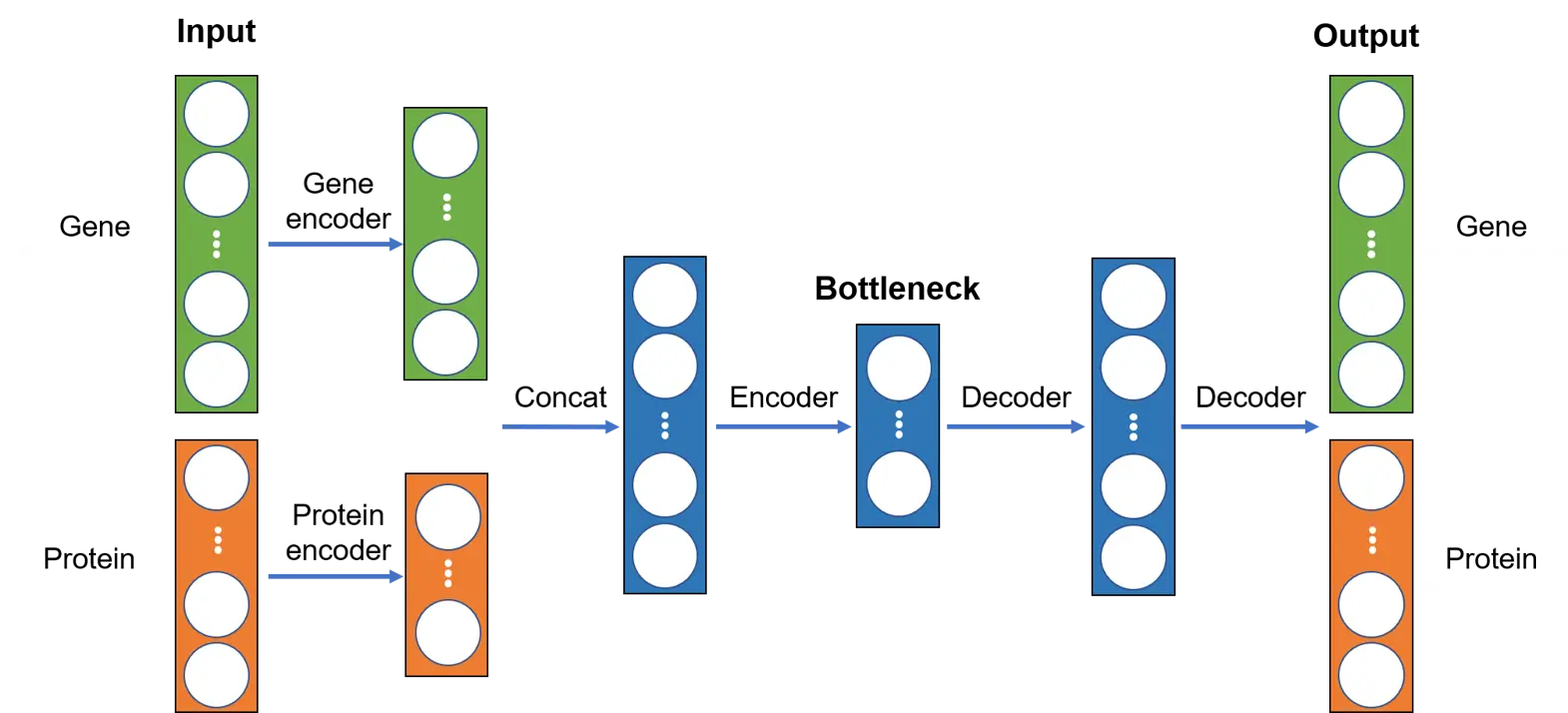
Since gene and protein data have dramatically different dimensions, we will first encode them separately using two different encoders and then concatenate the outputs, which will be passed through another encoder to generate the bottleneck layer. Subsequently, the decoder will try to reconstruct the input based on the bottleneck layer. The overall neural network architecture is illustrated below:

Image source- Eraslan et al Nat Rev Genet 2019

Autoencoder architecture for CITE-seq data

We use the module below to group linear, batchnorm, and dropout layers together in order to make it easier to implement encoder and decoder later:

class LinBnDrop(nn.Sequential):
    """Module grouping `BatchNorm1d`, `Dropout` and `Linear` layers, adapted from fastai."""
    
    def __init__(self, n_in, n_out, bn=True, p=0., act=None, lin_first=True):
        layers = [nn.BatchNorm1d(n_out if lin_first else n_in)] if bn else []
        if p != 0: layers.append(nn.Dropout(p))
        lin = [nn.Linear(n_in, n_out, bias=not bn)]
        if act is not None: lin.append(act)
        layers = lin+layers if lin_first else layers+lin
        super().__init__(*layers)

We start by implementing the encoder, which consists of three fully connected layer groups, one for RNA, one for protein, and one for the concatenated output that generates the latent representation of size latent_dim stored in the bottlenect layer.

class Encoder(nn.Module):
    """Encoder for CITE-seq data"""
    def __init__(self,
                 nfeatures_rna: int,
                 nfeatures_pro: int,
                 hidden_rna: int,
                 hidden_pro: int,
                 latent_dim: int,
                 p: float = 0):
        super().__init__()
        self.nfeatures_rna = nfeatures_rna
        self.nfeatures_pro = nfeatures_pro
        hidden_dim = hidden_rna + hidden_pro
        
        self.encoder_rna = nn.Sequential(
            LinBnDrop(nfeatures_rna, nfeatures_rna // 2, p=p, act=nn.LeakyReLU()),
            LinBnDrop(nfeatures_rna // 2, hidden_rna, act=nn.LeakyReLU())
        )
        self.encoder_protein = LinBnDrop(nfeatures_pro, hidden_pro, p=p, act=nn.LeakyReLU())
        self.encoder = LinBnDrop(hidden_dim, latent_dim, act=nn.LeakyReLU())

    def forward(self, x):
        x_rna = self.encoder_rna(x[:, :self.nfeatures_rna])
        x_pro = self.encoder_protein(x[:, self.nfeatures_rna:])
        x = torch.cat([x_rna, x_pro], 1)
        return self.encoder(x)

The decoder is a flipped version of the encoder.

class Decoder(nn.Module):
    """Decoder for CITE-seq data"""
    def __init__(self,
                 nfeatures_rna: int,
                 nfeatures_pro: int,
                 hidden_rna: int,
                 hidden_pro: int,
                 latent_dim: int):
        super().__init__()
        hidden_dim = hidden_rna + hidden_pro
        out_dim = nfeatures_rna + nfeatures_pro
        
        self.decoder = nn.Sequential(
            LinBnDrop(latent_dim, hidden_dim, act=nn.LeakyReLU()),
            LinBnDrop(hidden_dim, out_dim // 2, act=nn.LeakyReLU()),
            LinBnDrop(out_dim // 2, out_dim, bn=False)
            )

    def forward(self, x):
        return self.decoder(x)

Next, we assemble the encoder and decoder into an autoencoder, which is defined as a PyTorch Lightning Module to simplify the training process. We will define the following:

__init__ for creating and saving parameters and model
forward: for inference, which we will use to generate latent representations for downstream analysis
configure_optimizers for creating the optimizer and learning rate scheduler
training_step for calculating the loss (mean squared error (MSE) for our example) of a single batch
validation_step similar to training_step but on the validation set
test_step same as validation_step but on a test set.

class CiteAutoencoder(pl.LightningModule):
    def __init__(self,
                 nfeatures_rna: int,
                 nfeatures_pro: int,
                 hidden_rna: int,
                 hidden_pro: int,
                 latent_dim: int,
                 p: float = 0,
                 lr: float = 0.1):
        """ Autoencoder for citeseq data """
        super().__init__()
        
        # save hyperparameters
        self.save_hyperparameters()
 
        self.encoder = Encoder(nfeatures_rna, nfeatures_pro, hidden_rna, hidden_pro, latent_dim, p)
        self.decoder = Decoder(nfeatures_rna, nfeatures_pro, hidden_rna, hidden_pro, latent_dim)
        
        # example input array for visualizing network graph
        self.example_input_array = torch.zeros(256, nfeatures_rna + nfeatures_pro)

    def forward(self, x):
        # extract latent embeddings
        z = self.encoder(x)
        return z
    
    def configure_optimizers(self):
        optimizer = optim.Adam(self.parameters(), lr=self.hparams.lr)
        scheduler = optim.lr_scheduler.ReduceLROnPlateau(optimizer)
        return {"optimizer": optimizer, "lr_scheduler": scheduler, "monitor": "val_loss"}
    
    def _get_reconstruction_loss(self, batch):
        """ Calculate MSE loss for a given batch. """
        x, _ = batch
        z = self.encoder(x)
        x_hat = self.decoder(z)
        # MSE loss
        loss = F.mse_loss(x_hat, x)
        return loss
    
    def training_step(self, batch, batch_idx):
        loss = self._get_reconstruction_loss(batch)
        self.log("train_loss", loss)
        return loss
    
    def validation_step(self, batch, batch_idx):
        loss = self._get_reconstruction_loss(batch)
        self.log("val_loss", loss)
        
    def test_step(self, batch, batch_idx):
        loss = self._get_reconstruction_loss(batch)
        self.log("test_loss", loss)

Training the model

We will take advantage of the Trainer API from PyTorch Lightning to execute the training process. The two functions that we will be using are:

fit: Train a lightning module using the given train dataloader, and validate on the provided validation dataloader.
test: Test the given model on the provided dataloader.

def train_citeseq(hidden_rna: int = 30, hidden_pro: int = 18,
                  latent_dim: int = 24, p: float = 0.1, lr: float = 0.1):
    trainer = pl.Trainer(default_root_dir=CHECKPOINT_PATH,
                         gpus=1 if "cuda" in str(device) else 0,
                         max_epochs=50,
                         callbacks=[ModelCheckpoint(save_weights_only=True, mode="min", monitor="val_loss"),
                                    LearningRateMonitor("epoch")])
    trainer.logger._log_graph = True
    trainer.logger._default_hp_metric=None
    
    model = CiteAutoencoder(nfeatures_rna,
                            nfeatures_pro,
                            hidden_rna=hidden_rna,
                            hidden_pro=hidden_pro,
                            latent_dim=latent_dim,
                            p=p,
                            lr=lr)
    trainer.fit(model, train_dl, val_dl)
    
    train_result = trainer.test(model, train_dl, verbose=False)
    val_result = trainer.test(model, val_dl, verbose=False)
    test_result = trainer.test(model, test_dl, verbose=False)
    result = {"train": train_result, "val": val_result, "test": test_result, }
    return model, result

model, result = train_citeseq()

print(f"Training loss:  {result['train'][0]['test_loss']:.3f}")
print(f"Validation loss:  {result['val'][0]['test_loss']:.3f}")
print(f"Test loss: {result['test'][0]['test_loss']:.3f}")

PyTorch Lightning automatically logs the training results into TensorBoard, which we can open like below:

%tensorboard --host 0.0.0.0 --port 8000 --logdir saved_models/lightning_logs/version_0

# kill tensorboard process
!kill $(ps -e | grep 'tensorboard' | awk '{print $1}')

Visualize latent representations

The latent space in our example has 24 dimensions. In order to visualize and inspect how different types of immune cells cluster in the latent space, we first use the trained model to generate the latent representations of the test dataset and then use UMAP, which is widely used in single-cell analysis, to reduce the dimensions for visualization in 2D.

test_encodings = []
test_labels = []
    
model.eval()
with torch.no_grad():    
    for x, y in tqdm(test_dl, desc="Encoding cells"):
        test_encodings.append(model(x.to(model.device)))
        test_labels += y.to(torch.int).tolist()
        
test_embeds = torch.cat(test_encodings, dim=0).cpu().numpy()
test_labels = le.inverse_transform(test_labels)

# run umap for dimensionality reduction and visualization
embeds_umap = umap.UMAP(random_state=0).fit_transform(test_embeds)

# visualize umap
fig = px.scatter(x=embeds_umap[:, 0], y=embeds_umap[:, 1], color=test_labels, width=800, height=600,
                 labels={
                     "x": "UMAP1",
                     "y": "UMAP2",
                     "color": "Cell type"}
                )
fig.show(renderer="colab")

We can also visualize and explore latent representations using TensorBoard, which provides a convinient interface for popular dimensionality reduction methods such as UMAP, TSNE, and PCA.

# visualization with tensorboard
writer = SummaryWriter("tensorboard/")
writer.add_embedding(test_embeds, metadata=test_labels)

# wait for saving files
time.sleep(3)

%tensorboard --host 0.0.0.0 --port 8000 --logdir  tensorboard/

writer.close()

# kill tensorboard process
!kill $(ps -e | grep 'tensorboard' | awk '{print $1}')

Summary

Credit: Yuan Tian

About Saturn Cloud

Saturn Cloud is your all-in-one solution for data science & ML development, deployment, and data pipelines in the cloud. Spin up a notebook with 4TB of RAM, add a GPU, connect to a distributed cluster of workers, and more. Request a demo today to learn more.

Start for free