How to Use Pandas with Jupyter Notebooks

How to Use Pandas with Jupyter Notebooks

If you are a data scientist, you are likely familiar with both Pandas and Jupyter Notebooks. Pandas is a popular Python library for data manipulation and analysis, while Jupyter Notebooks are a web-based interactive computing environment that allows you to create and share documents containing live code, equations, visualizations, and narrative text. In this blog post, we will explore how to use Pandas with Jupyter Notebooks to analyze and manipulate data.

Getting Started with Pandas and Jupyter Notebooks

Before we dive into the details of how to use Pandas with Jupyter Notebooks, let’s make sure we have everything set up correctly. First, make sure you have both Pandas and Jupyter Notebooks installed on your computer. You can do this by running the following commands in your terminal:

pip install pandas
pip install jupyter

Once you have both Pandas and Jupyter Notebooks installed, you can launch Jupyter Notebooks by running the following command in your terminal:

jupyter notebook

This will open up a web browser and take you to the Jupyter Notebook dashboard. From here, you can create a new notebook by clicking on the “New” button in the top right corner and selecting “Python 3” under “Notebook”.

Importing Pandas

Now that we have our Jupyter Notebook set up, let’s import Pandas into our notebook. To do this, simply run the following code in a new cell:

import pandas as pd

This will import Pandas into our notebook and allow us to use all of its functions and methods.

Loading Data into Pandas

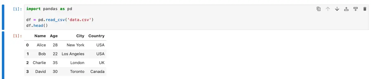
The first step in analyzing data with Pandas is to load the data into a Pandas DataFrame. There are many ways to do this, but one of the most common is to load data from a CSV file. To do this, we can use the read_csv() function in Pandas. For example, if we have a CSV file called “data.csv” in the same directory as our Jupyter Notebook, we can load it into a DataFrame like this:

df = pd.read_csv('data.csv')

This will create a new DataFrame called df that contains all of the data from the CSV file.

Exploring Data with Pandas

Now that we have our data loaded into a Pandas DataFrame, we can start exploring it. One of the most useful functions for exploring data is the head() function, which allows us to see the first few rows of the DataFrame. For example, if we want to see the first five rows of our DataFrame, we can run the following code:

df.head()

This will display the first five rows of our DataFrame.

Another useful function for exploring data is the describe() function, which provides summary statistics for each column in the DataFrame. For example, if we want to see summary statistics for our DataFrame, we can run the following code:

df.describe()

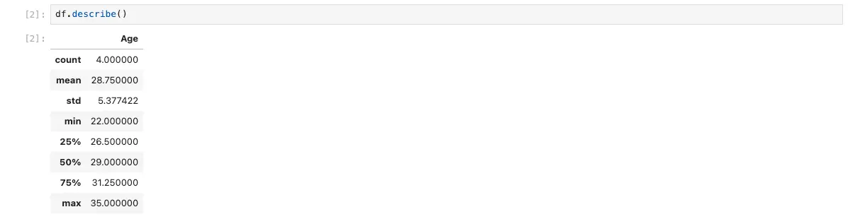
This will display summary statistics for each column in our DataFrame.

Manipulating Data with Pandas

Once we have explored our data, we may want to manipulate it in some way. Pandas provides a wide range of functions and methods for manipulating data, but we will only cover a few of the most common ones here.

Selecting Columns

To select a single column from a DataFrame, we can use the square bracket notation. For example, if we have a column called “age” in our DataFrame, we can select it like this:

df['age']

This will return a new Series object that contains only the “age” column.

To select multiple columns, we can pass a list of column names to the square bracket notation. For example, if we have columns called “age” and “income” in our DataFrame, we can select them like this:

df[['age', 'income']]

This will return a new DataFrame that contains only the “age” and “income” columns.

Filtering Rows

To filter rows based on a condition, we can use the square bracket notation with a boolean expression. For example, if we want to select only the rows where the “age” column is greater than 30, we can run the following code:

df[df['age'] > 30]

This will return a new DataFrame that contains only the rows where the “age” column is greater than 30.

Grouping Data

To group data by a particular column and perform an aggregation function on each group, we can use the groupby() function. For example, if we want to group our data by the “gender” column and calculate the mean age for each gender, we can run the following code:

df.groupby('gender')['age'].mean()

This will return a new Series object that contains the mean age for each gender.

Conclusion

In this blog post, we have explored how to use Pandas with Jupyter Notebooks to analyze and manipulate data. We have covered the basics of loading data into a Pandas DataFrame, exploring data with Pandas, and manipulating data with Pandas. While this is just the tip of the iceberg when it comes to what Pandas can do, it should give you a good starting point for working with data in Python.

SHARE:

About Saturn Cloud

Saturn Cloud is your all-in-one solution for data science & ML development, deployment, and data pipelines in the cloud. Spin up a notebook with 4TB of RAM, add a GPU, connect to a distributed cluster of workers, and more. Request a demo today to learn more.