A walkthrough of the layers involved in turning NVIDIA Dynamo into a multi-tenant, per-token inference service.
This is Part 3. Part 1 laid out the three planes of an inference stack (data, control, tenant). Part 2 covered NVIDIA Dynamo: what it does and where it fits. This post is the build: how to stand up a multi-tenant, per-token inference service on Dynamo, layer by layer.
What “token factory” means here
A token factory is an inference service that meters and bills per token, across many tenants, over many models. A customer hits an OpenAI-compatible endpoint with a model= name, gets a completion, and is billed for exactly the tokens they used at the right price for that model, and the same service does that for many customers, many base models, and many fine-tuned adapters at once.
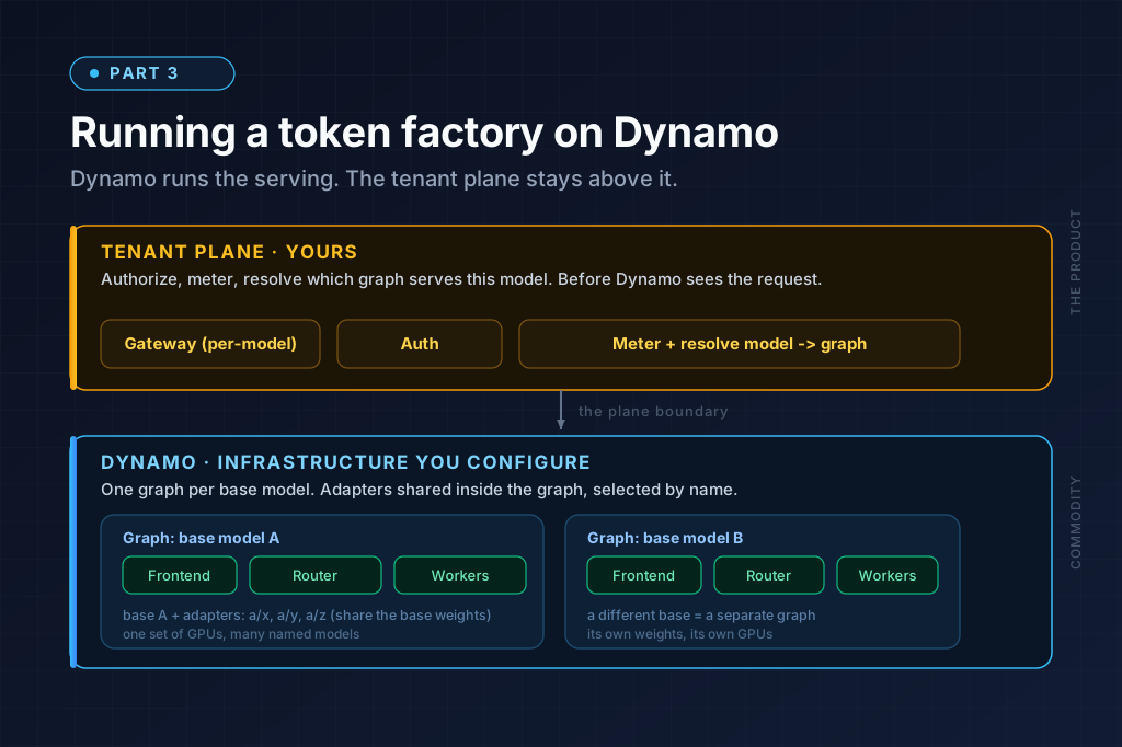
Dynamo is the right foundation for this. It is a genuinely strong piece of infrastructure: a multi-node serving system with KV-aware routing, prefill/decode disaggregation, and SLA-driven autoscaling, and you should absolutely build on it rather than reinvent any of that. It owns the data plane (routing, KV cache, disaggregation, autoscaling) and the control plane (the operator and CRDs). It is also clear about its boundary: in NVIDIA’s own words, it “has no concept of your customers, your billing, or your quotas.”
So a token factory is Dynamo plus the layers around it that turn a serving system into a metered, multi-tenant product. Here is the full stack, bottom-up.
Layer 1: the cluster Dynamo runs on
Set this up once per cluster, before any model serves a request:
- The Dynamo Operator, installed via Helm. It watches the Dynamo CRDs and reconciles them into pods (Frontend, Router, workers), wiring up service discovery, GPU resource requests, and multi-node placement. It also handles the image-pull secret for the runtime container.
- A coordination backend. This is where workers register and where the router’s cache-state events flow. Depending on the Dynamo version it is either an external etcd (with NATS optional, for event-backed KV routing rather than the prediction-based mode), or a newer Kubernetes-native event plane that removes the external dependency. Confirm which your pinned version uses, running etcd and NATS as stateful services is real operational surface, so the native path is worth preferring where it is available.
- GPU node pools sized to the base models you intend to offer. Add RDMA-capable networking (InfiniBand, RoCE, or NVLink) only if you plan to use disaggregated prefill/decode; the aggregated default does not need it (see Layer 3).
- Secrets: the image-pull credential for the Dynamo runtime image, and a HuggingFace token for pulling gated base-model weights. The HF token is referenced by name from the graph CRDs, so provision it into the serving namespace before the first graph applies.
- A shared model cache, typically a ReadWriteMany PVC, so a multi-gigabyte base model is downloaded once cluster-wide and mounted read-only by every replica of every graph that uses it, rather than re-pulled per pod. Without this, each new replica of a large base pays a cold-start download of tens of gigabytes.
Follow Dynamo’s deployment guide and this comes together as a standard bring-up. It is the foundation the rest of the stack stands on.
Layer 2: the serving graphs
The unit is a DynamoGraphDeployment (a “graph”), and one rule shapes everything above it:
A graph serves exactly one base model. The multi-LoRA exception is the efficiency story: one graph loads a base model once and serves many fine-tuned adapters off it by name, because the adapters share the base weights. The sharing boundary is per base model:
- Many adapters of the same base model go on one graph. The base loads once; each adapter is a few hundred megabytes. An organization with five fine-tunes of one base runs on one set of GPUs.
- Different base models go on separate graphs. A worker holds one base model’s weights, so a Llama base and a Mistral base are two graphs.
One caveat to check before you commit to this: in Dynamo, multi-LoRA is a vLLM-backend feature. Dynamo’s own feature matrix lists LoRA as supported on vLLM and not on SGLang or TensorRT-LLM. If your plan was to serve a flagship base on TensorRT-LLM for peak throughput, the adapter-sharing economics in this section do not apply to that backend; you would serve each fine-tune of it as its own full model. So the “many adapters, one base, one set of GPUs” win is a reason to serve your fine-tune bases on vLLM.
Configuring a graph is two layers of settings: the Dynamo layer (component topology, replica counts, GPU counts, placement) and the engine layer (the vLLM arguments passed straight through). A minimal aggregated graph for a LoRA-serving base looks like this:
apiVersion: nvidia.com/v1alpha1
kind: DynamoGraphDeployment
metadata:
  name: llama-3-1-8b
spec:
  services:
    Frontend:
      componentType: frontend
      replicas: 1
    VllmWorker:
      componentType: worker
      replicas: 2
      resources:
        limits: { gpu: "1" }
      extraPodSpec:
        mainContainer:
          command: ["python3", "-m", "dynamo.vllm"]
          args:
            - "--model"
            - "meta-llama/Llama-3.1-8B-Instruct"
            - "--enable-lora"
            - "--max-loras"
            - "8"          # adapters resident per worker at once
            - "--max-lora-rank"
            - "32"
The Frontend is the OpenAI-compatible entry point and the KV-aware router; the VllmWorker block is where your existing vLLM configuration lives, unchanged. --enable-lora, --max-loras, --max-lora-rank, --tensor-parallel-size, and --quantization mean exactly what they mean in a raw vllm serve command. If you already tune these, that knowledge moves directly into the engine-args block.
Adapters are not baked into the graph. Once the base graph is running, each fine-tune is registered with a separate DynamoModel resource that names the base and the adapter’s source URI:
apiVersion: nvidia.com/v1alpha1
kind: DynamoModel
metadata:
  name: acme-support-v3
spec:
  baseModelName: meta-llama/Llama-3.1-8B-Instruct
  source: s3://tenant-adapters/acme/support-v3/
The operator discovers every worker pod running that baseModelName, loads the adapter onto all of them, and exposes it under its name. This is what closes a gap you would otherwise hit with raw vLLM, where an adapter loaded via the API lands on one replica and is missing from the others behind the load balancer. With DynamoModel, the fan-out to every replica of the base is the operator’s job.
Layer 3: the serving-config decisions
Each base model needs a set of choices. Part 2 has the reasoning; here is what you decide per model, and how it lands in the graph:
- Aggregated or disaggregated. Aggregated runs prefill and decode in one worker (the single
VllmWorkerabove). Disaggregated splits them into separateVllmPrefillWorkerandVllmDecodeWorkerservices and moves the KV cache between them, which needs an RDMA fabric to be worth it. Start aggregated. NVIDIA cites throughput gains up to roughly 7x from disaggregation, but that is a ceiling under favorable workload and fabric conditions, not a planning input; treat it as “worth measuring on RDMA-capable hardware,” not as guaranteed headroom. - Parallelism. Dense models (Llama, Mistral) set
--tensor-parallel-sizeto the number of GPUs needed to hold weights plus KV cache (one for an 8B model, more as the model grows), then scale throughput by adding workerreplicasrather than widening tensor parallelism, because decode favors many concurrent sequences. MoE models (DeepSeek-class) instead use wide expert parallelism with--enable-expert-parallel, data-parallel attention, and an expert load balancer, a distinct configuration worth treating as its own model class. Multimodal models add an encode phase in front of prefill. - Quantization.
--quantization(FP8 and similar) roughly halves the memory footprint of weights and KV cache, which directly raises how many concurrent requests and how many adapters fit on a GPU. For a fine-tune-serving base, this often decides whether a model class fits on one GPU or needs two. - Autoscaling. Pick one mode per graph. The SLA-based Planner takes latency targets (TTFT and ITL) plus floor and ceiling replica bounds and owns the replica count, forecasting load to scale prefill and decode pools ahead of demand. The floor keeps warm capacity so requests do not cold-start from zero; the ceiling caps cost. In an autoscaled mode you set the SLOs and the bounds, never a raw replica count, because the Planner owns that number. The floor is a direct cost dial, not a free latency win: a warm replica bills for its GPUs whether or not it serves a token, which is the hinge the next section is about.
The economics under all of it
Before the request path, one thing that sits under every layer and is not a plumbing problem: the unit economics. You buy GPUs by the hour and sell tokens by the million, and the gap between those two units is your margin. It is set almost entirely by utilization, and no amount of correct engineering above the serving layer improves a low duty cycle.
The arithmetic is worth doing before you write any code. A GPU has a cost per hour and a peak token throughput for a given model. Multiply throughput by an hour and you get the tokens that GPU could produce; divide the hourly cost by that and you get your cost per million tokens at full utilization. Then multiply by your realistic duty cycle. A model that pencils out at full load can be deeply underwater at 30% utilization, and 30% is a normal number for a service with spiky, per-tenant traffic and warm floor replicas holding capacity for latency.
This is where several earlier choices show up as money:
- Warm floor replicas buy you low tail latency and cost you idle GPU-hours. That trade is a business decision per model, not a default to leave on. A model with steady traffic can carry a floor; a long-tail fine-tune with occasional traffic probably should scale to zero and accept a cold start.
- Shared graphs are the main lever in your favor. Packing many adapters of one base onto one set of GPUs is what turns a fleet of individually-underutilized fine-tunes into one well-utilized base. The per-base sharing boundary from Layer 2 is a margin mechanism, not just a deployment convenience.
- Quantization and right-sized tensor parallelism change the denominator: more concurrent requests per GPU is directly more sellable tokens per GPU-hour.
The point is that a token factory’s viability is decided at this layer, not the ones above it. Model the blended cost per million tokens at a duty cycle you actually believe, per model, before committing to a price. The plumbing in the next two sections is what makes the service correct and multi-tenant; the numbers here are what make it a business.
Layer 4: the request path
Above the serving graphs, every request passes through several steps before it reaches a Dynamo Frontend:
client
  -> ingress / gateway        (per-model route, TLS)
  -> authorization            (may this caller use this resource?)
  -> metering + resolution     (which graph serves this model? record usage)
  -> Dynamo Frontend           (the graph for this model's base)
  -> Router -> Worker          (base model + the named adapter)
The bottom two hops are Dynamo. The top three you provide:
Authorization. Dynamo serves any model= name a graph knows about to anyone who can reach its Frontend. In front of it sits an identity system that maps a caller’s API key to a tenant, a record of which models each tenant may use, and a check that runs on every request. A common structure is a per-model route (one subdomain or path per model) fronted by a forward-auth step that authorizes the token for that specific resource and injects a verified tenant identity header the downstream steps can trust. That header is what ties the request to a tenant for both access control and billing.
Model-name routing. One graph serves one base model but many named models (every adapter, plus the bare base), and a deployment has many graphs, so an incoming model= name has to be resolved to the correct graph’s Frontend Service. That means a resolution table mapping each served model name to its {tenant, base model, adapter, upstream Service}, kept in sync as models are created and deleted, and consulted on the hot path of every request. The lookup has to be fast (a routing decision is measured against a completion that takes seconds, so it must add no meaningful latency) and correct (a stale entry routes a live request to the wrong graph). Dynamo does not do this cross-graph dispatch; the resolution layer is yours.
Metering. OpenAI-compatible engines return a usage block with prompt_tokens, completion_tokens, and cached-token counts. For streamed responses (most of them) that block arrives in the final chunk, so the metering point has to read the stream to completion to capture it, and with many engines you must set stream_options.include_usage=true or the counts come back null. It also has to handle the client hanging up mid-stream: the GPU did the work for the tokens generated before the disconnect, so partial usage is captured on the abort path rather than dropped. Each usage record is attributed to the tenant from the auth header, keyed with an idempotency id so a retried emission is not double-counted, and written to a durable event stream off the hot path. Because one graph now serves many models, the price key is resolved per request from the model name in the body, not stamped once per deployment as it would be with one model per pod; the same read that resolves the model for routing resolves it for the price key.
Layer 5: the tenant plane
Around the request path sits the rest of the product:
- Model lifecycle. Creating a model becomes find-or-create the graph for its base model, then apply a
DynamoModelto register the adapter, rather than “deploy one container per model.” Starting a model on a shared base is registering its adapter; stopping it is deleting that oneDynamoModelso Dynamo stops serving it while the graph keeps running for every other tenant on the same base. The underlying GPUs scale to zero only when the last adapter on a base leaves. Deleting a model deregisters the adapter and, if it was the last one, tears the graph down. Each of these maps a customer-facing “start / stop / delete model” action onto the right sequence of CRD operations, without disturbing co-tenants. - Quotas and fairness. Real-time spend and rate limits, plus fairness across the tenants sharing one graph’s GPUs. These are two different systems: enforcement needs a fast, approximate running counter you check before forwarding a request and that can self-correct, while billing needs the durable, reconciled event stream and cannot be approximate. Serving both from one path gives you either slow enforcement or unreliable billing.
- Billing. The durable usage events become invoices, applying per-model and per-tier prices, supporting cached-token rates that differ from fresh-input rates, and keeping an auditable separation between what was metered and what was charged so you can re-rate or issue credits without re-capturing usage.
- The customer-facing surface. Usage dashboards, request and response logs with their own retention and privacy rules, model management, and API-key issuance, all mapping your real tenants onto whatever identity objects the gateway, the resolution table, and the engine each use, and keeping those in sync as tenants are created, suspended, and rotated.
Multi-tenant isolation on shared GPUs
Sharing a base model’s GPUs across tenants is the economics of Layer 2, and it puts different tenants inside one serving process. Three concerns follow that a single-tenant deployment never has.
Adapter weights are tenant-controlled input. A DynamoModel points at an adapter URI the tenant produced, and registering it loads those weights into your serving process. That is untrusted input crossing into your runtime, so the load path needs the same discipline as any upload: accept a safetensors-style format that is data, not arbitrary pickled code; validate shapes and rank against what the base expects; and scan before loading. An adapter that fails validation should be rejected at registration, not discovered at serve time.
Prefix caching is a cross-tenant surface, and the default handling is partial. Prefix caching reuses KV blocks across requests, and on a shared base that means across tenants. vLLM mixes the LoRA adapter’s identity into each block’s hash, so two different adapters cannot collide on a cached block even for identical token sequences; the per-adapter case is closed. What is not closed by that alone is the bare base model that many tenants call directly: identical prompt prefixes there can share blocks, and cache-hit timing is observable, which is a classic side channel. vLLM’s mechanism for this is a per-request cache_salt: requests carrying the same salt may share cached blocks, requests with different salts cannot. Setting the salt per tenant (or per isolation domain) on requests to a shared base turns the side channel off, at the cost of the cross-tenant cache sharing you were giving up anyway for isolation. This is a decision to make deliberately per model, not a default to inherit.
The engine has no per-tenant fairness. vLLM’s scheduler batches by what maximizes throughput, not by who is calling. One tenant submitting a 100k-token prefill on a shared graph raises the inter-token latency for every other tenant on it until that prefill drains. Nothing inside the engine prevents this, so the fairness has to live above it: admission control that caps per-tenant in-flight work or long-prompt concurrency on a shared graph, before the request reaches the Frontend. This is more than the one “fairness” bullet in Layer 5 suggests, and it is the kind of thing you tune with real traffic rather than get right on the first pass.
None of these are reasons not to share GPUs; sharing is the whole margin story. They are the work that makes sharing safe, and they are specific to running many tenants on one model rather than one.
What Dynamo gives you, and what sits around it
| Dynamo gives you | The layers around it |
|---|---|
| KV-aware routing within a graph | Which graph a request goes to |
| Adapter load/unload across replicas | Who may register and use an adapter, and validating its weights |
| SLA-based autoscaling of a graph | Per-tenant quotas, fairness, admission control |
| OpenAI-compatible serving | Metering, billing, and the pricing model |
| Prefill/decode disaggregation | The customer-facing API, dashboards, and model lifecycle |
| Adapter-aware prefix cache hashing | Cross-tenant cache isolation on shared base models |
The left column is why you build on Dynamo: a multi-node router, a KV-transfer path, and an SLA autoscaler, all done well and ready to configure. The right column is the token factory around it, plus the unit economics underneath all of it.
Where to start
The layer map above is the build. Layers 1 through 3 are Dynamo: install it, define your graphs, choose the serving config. Layers 4 and 5 are the request path and the tenant plane, the authorization, per-request routing, metering, quotas, billing, lifecycle, and customer surface that turn the serving system into a product. Some of the upper layers you assemble rather than write from scratch: authorization can be a forward-auth filter in front of the gateway, rating and invoicing are what billing platforms exist for, and the resolution table is a small service with a cache. The genuinely custom piece is a streaming-aware metering path that survives client aborts and emits idempotent usage events.
What makes this work is less the code than the properties around it. Metering runs on money, and metering bugs are silent: they surface months later as disputed invoices, so the abort path and the idempotency key earn more care than their line count suggests. Multi-tenant isolation on shared GPUs is a correctness-and-security property, not a feature. And once it is serving customers, the whole thing has to hold an SLO on-call. None of that is algorithmically novel, and all of it is the difference between a demo and a service.
At Saturn Cloud, those upper layers are already built and run in production. If you are standing up a token factory, you can build them, the map above is a fair checklist, or you can start from a stack where Layers 4 and 5 exist and the economics and isolation work is done, and put your time into the models and the service you are actually offering. Either way, Dynamo is the right engine underneath, and the map above is what surrounds it.
This is Part 3 of a series. See Part 1: What an LLM Inference Stack Actually Looks Like and Part 2: Where NVIDIA Dynamo Fits in an Inference Stack.